
Maximization Without Calculus: Methods and Applications
E N D
Presentation Transcript
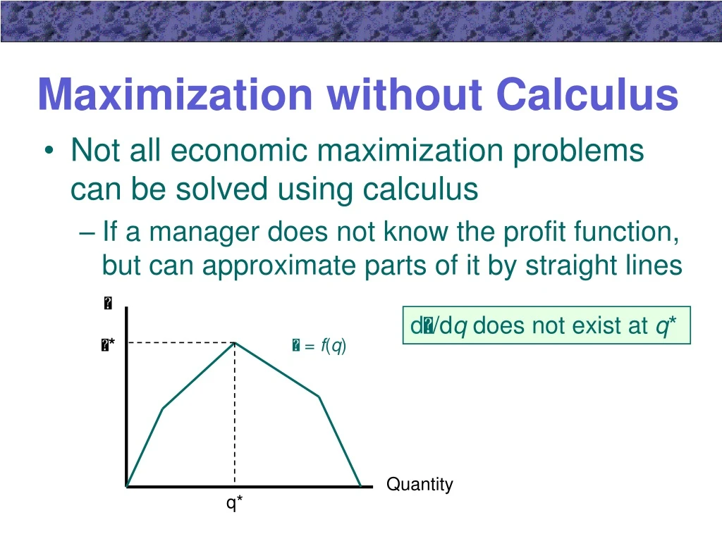
Maximization without Calculus • Not all economic maximization problems can be solved using calculus • If a manager does not know the profit function, but can approximate parts of it by straight lines d/dq does not exist at q* * = f(q) Quantity q*
Maximization without Calculus • Calculus also cannot be used in the case where a firm cannot produce fractional values of output • d/dq does not exist at q*
Second Order Conditions - Functions of One Variable • Let y = f(x) • A necessary condition for a maximum is that dy/dx = f ’(x) = 0 • To ensure that the point is a maximum, y must be decreasing for movements away from it
Second Order Conditions - Functions of One Variable • The total differential measures the change in y dy = f ‘(x) dx • To be at a maximum, dy must be decreasing for small increases in x • To see the changes in dy, we must use the second derivative of y
Second Order Conditions - Functions of One Variable • Note that d 2y < 0 implies that f ’’(x)dx2 < 0 • Since dx2 must be positive, f ’’(x) < 0 • This means that the function f must have a concave shape at the critical point
Second Order Conditions - Functions of Two Variables • Suppose that y = f(x1, x2) • First order conditions for a maximum are y/x1 = f1 = 0 y/x2 = f2 = 0 • To ensure that the point is a maximum, y must diminish for movements in any direction away from the critical point
Second Order Conditions - Functions of Two Variables • The slope in the x1 direction (f1) must be diminishing at the critical point • The slope in the x2 direction (f2) must be diminishing at the critical point • But, conditions must also be placed on the cross-partial derivative (f12 = f21) to ensure that dy is decreasing for all movements through the critical point
Second Order Conditions - Functions of Two Variables • The total differential of y is given by dy = f1 dx1 + f2 dx2 • The differential of that function is d 2y = (f11dx1 + f12dx2)dx1 + (f21dx1 + f22dx2)dx2 d 2y = f11dx12 + f12dx2dx1 + f21dx1 dx2 + f22dx22 • By Young’s theorem, f12 = f21 and d 2y = f11dx12 + 2f12dx2dx1 + f22dx22
Second Order Conditions - Functions of Two Variables d 2y = f11dx12 + 2f12dx2dx1 + f22dx22 • For this equation to be unambiguously negative for any change in the x’s, f11 and f22 must be negative • If dx2 = 0, then d 2y = f11dx12 • For d 2y < 0, f11 < 0 • If dx1 = 0, then d 2y = f22dx22 • For d 2y < 0, f22 < 0
Second Order Conditions - Functions of Two Variables d 2y = f11dx12 + 2f12dx2dx1 + f22dx22 • If neither dx1 nor dx2 is zero, then d 2y will be unambiguously negative only if f11 f22 - f122 > 0 • The second partial derivatives (f11 and f22) must be sufficiently large that they outweigh any possible perverse effects from the cross-partial derivatives (f12 = f21)
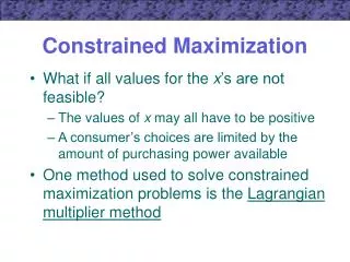
Constrained Maximization • Suppose we want to choose x1 and x2 to maximize y = f(x1, x2) • subject to the linear constraint c - b1x1 - b2x2 = 0 • We can set up the Lagrangian L = f(x1, x2) - (c - b1x1 - b2x2)
Constrained Maximization • The first-order conditions are f1 - b1 = 0 f2 - b2 = 0 c - b1x1 - b2x2 = 0 • To ensure we have a maximum, we must use the “second” total differential d 2y = f11dx12 + 2f12dx2dx1 + f22dx22
Constrained Maximization • Only the values of x1 and x2 that satisfy the constraint can be considered valid alternatives to the critical point • Thus, we must calculate the total differential of the constraint -b1dx1 - b2dx2 = 0 dx2 = -(b1/b2)dx1 • These are the allowable relative changes in x1 and x2
Constrained Maximization • Because the first-order conditions imply that f1/f2 = b1/b2, we can substitute and get dx2 = -(f1/f2) dx1 • Since d 2y = f11dx12 + 2f12dx2dx1 + f22dx22 we can substitute for dx2 and get d 2y = f11dx12 - 2f12(f1/f2)dx1 + f22(f12/f22)dx12
Constrained Maximization • Combining terms and rearranging d 2y = f11 f22- 2f12f1f2 + f22f12 [dx12/ f22] • Therefore, for d 2y < 0, it must be true that f11 f22- 2f12f1f2 + f22f12 < 0 • This equation characterizes a set of functions termed quasi-concave functions • Any two points within the set can be joined by a line contained completely in the set
Constrained Maximization • Recall the fence problem: Maximize A = f(x,y) = xy subject to the constraint P - 2x - 2y = 0 • Setting up the Lagrangian [L = x·y + (P - 2x - 2y)] yields the following first-order conditions: L/x = y - 2 = 0 L/y = x - 2 = 0 L/ = P - 2x - 2y = 0
Constrained Maximization • Solving for the optimal values of x, y, and yields x = y = P/4 and = P/8 • To examine the second-order conditions, we compute f1 = fx= y f2 = fy = x f11 = fxx = 0 f12 = fxy = 1 f22 = fyy = 0
Constrained Maximization • Substituting into f11 f22- 2f12f1f2 + f22f12 we get 0 ·x2 - 2 ·1 ·y ·x + 0 ·y2 = -2xy • Since x and y are both positive in this problem, the second-order conditions are satisfied