Download
1 / 22
330 likes | 697 Views
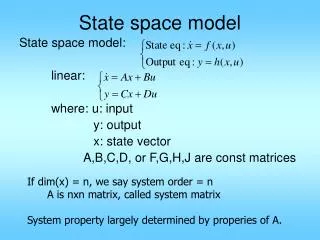
State space model. State space model: linear: where: u: input y: output x: state vector A,B,C,D, or F,G,H,J are const matrices. If dim(x) = n, we say system order = n A is nxn matrix, called system matrix System property largely determined by properies of A.

E N D
State space model State space model: linear: where: u: input y: output x: state vector A,B,C,D, or F,G,H,J are const matrices If dim(x) = n, we say system order = n A is nxn matrix, called system matrix System property largely determined by properies of A.
State transition matrix: eAt • eAt is an nxn matrix • eAt =ℒ-1((sI-A)-1), or ℒ (eAt)=(sI-A)-1 • eAt= AeAt=eAtA • eAt = Inxn+At+ A2t2+ A3t3 + • eAt is invertible: (eAt)-1= e(-A)t • eA0=I • eAt1 eAt2= eA(t1+t2) def
I/O model to state space • Infinite many solutions, all equivalent. • Controller canonical form:
Example n=4 a3 a2 a1 a0 b1 b0=b2=b3=0
>> n=[1 2 3];d=[1 4 5 6]; >> [A,B,C,D]=tf2ss(n,d) A = -4 -5 -6 1 0 0 0 1 0 B = 1 0 0 C = 1 2 3 D = 0 >> tf(n,d) Transfer function: s^2 + 2 s + 3 --------------------- s^3 + 4 s^2 + 5 s + 6
Characteristic values • Char. eq of a system is det(sI-A)=0 the polynomial det(sI-A) is called char. pol. the roots of char. eq. are char. values they are also the eigen-values of A e.g. ∴ (s+1)(s+2)2 is the char. pol. (s+1)(s+2)2=0 is the char. eq. s1=-1,s2=-2,s3=-2 are char. values or eigenvalues
can ? set t=0 ∴No can ? √ at t=0: ? √
Solution of state space model Recall: sX(s)-x(0)=AX(s)+BU(s) (sI-A)X(s)=BU(s)+x(0) X(s)=(sI-A)-1BU(s)+(sI-A)-1x(0) x(t)=(ℒ-1(sI-A)-1))*Bu(t)+ ℒ-1(sI-A)-1) x(0) x(t)= eA(t-τ)Bu(τ)d τ+eAtx(0) y(t)= CeA(t-τ)Bu(τ)d τ+CeAtx(0)+Du(t)
S.S to T.F. X(s)=(sI-A)-1BU(s) Y(s)=C(sI-A)-1BU(s)+DU(s) =(D+ C(sI-A)-1B)U(s) ∴ T.F. H(s)= D+ C(sI-A)-1B In matlab: ss2tf eig roots poly use help to find out how to use these
In Matlab: >> A=[0 1;-2 -3]; >> B=[0;1]; >> C=[1 3]; >> D=[0]; >> [n,d]=ss2tf(A,B,C,D) n = 0 3.0000 1.0000 d = 1 3 2 >>tf(n,d)
But don’t use those for hand calculation use:X(s)=(sI-A)-1BU(s)+(sI-A)-1x(0) x(t)=ℒ-1{(sI-A)-1BU(s)}+{ℒ-1 (sI-A)-1} x(0) & Y(s)=C(sI-A)-1BU(s)+DU(s)+C(sI-A)-1x(0) y(t)= ℒ-1{C(sI-A)-1BU(s)+DU(s)}+C{ℒ-1 (sI-A)-1} x(0) e.g. u= unit step
Eigenvalues, eigenvectors Given a nxn square matrix A, p is an eigenvector of A if Ap∝p i.e. λ s.t. Ap= λp λis an eigenvalue of A Example: , Let , ∴p1 is an e-vector, & the e-value=1 Let , ∴p2 is also an e-vector, assoc. with the λ =-2
In Matlab >> A=[2 0 1; 0 2 1; 1 1 4]; >> [P,D]=eig(A) P = 0.6280 0.7071 0.3251 0.6280 -0.7071 0.3251 -0.4597 -0.0000 0.8881 p1 p2 p3 D =1.2679 0 0 0 2.0000 0 0 0 4.7321 λ1 λ2 λ3
If we use [P,D]=eig(A) get approximate but wrong answer Should use: >>[P,J]=jordan(A) P = 0.3750 0 1 0.625 0 8 4 0 -0.375 0 0 0.375 0 16 9 0 J= -8 0 0 0 0 -16 1 0 0 0 -16 1 0 0 0 -16 a 3x3 Jordan block assoc. w/. λ=-16
In general, if λ, P is an e-pair for A, AP= λP λP-AP=0 λIP-AP=0 (λI-A)P=0 ∵ P≠0 ∴ det(λI-A)=0 ∴ λ is a sol. of char. eq of A • char. pol. of nxn A has deg=n ∴ A has n eigen-values. e.g. A= , det(λI-A)=(λ-1)(λ+2)=0 ⇒ λ1=1, λ2=-2
If λ1 ≠λ2 ≠λ3⋯ then the corresponding P1, P2, ⋯ will be linearly independent, i.e., the matrix P=[P1⋮P2 ⋮ ⋯Pn] will be invertible. AP1= λ1P1 AP2= λ2P2 ⋮ A[P1⋮P2 ⋮ ⋯]=[AP1⋮AP2 ⋮ ⋯] =[λ P1⋮ λ P2 ⋮ ⋯] =[P1 P2 ⋯]
∴ AP=PΛ P-1AP= Λ=diag(λ1, λ2, ⋯) ∴If A has n lin. ind. Eigenvectors then A can be diagonalized. Note: Not all square matrices can be diagonalized.
If A does not have n lin. ind. e-vectors (some of the eigenvalues are identical), then A can not be diagonalized E.g. A= det(λI-A)= λ4+56λ3+1152λ2+10240λ+32768 λ1=-8 λ2=-16 λ3=-16 λ4=-16 by solving (λI-A)P=0