Download
1 / 50
500 likes | 621 Views
Accuracy of Early GFS and ECMWF Sandy Track Forecasts: Evidence for a Dependence on Cumulus Parameterization . Nick Bassill Supported by DOE grant DEFG0208ER64557. Sample Track Differences. 0000 UTC 23 October. 1200 UTC 23 October. BLACK = Best Track RED = ECMWF BLUE = GFS.

E N D
Accuracy of Early GFS and ECMWF Sandy Track Forecasts: Evidence for a Dependence on Cumulus Parameterization Nick Bassill Supported by DOE grant DEFG0208ER64557
Sample Track Differences 0000 UTC 23 October 1200 UTC 23 October BLACK = Best Track RED = ECMWF BLUE = GFS 0000 UTC 24 October 1200 UTC 24 October
Best Track EPS GEFS From TIGGE archive (found at http://apps.ecmwf.int/datasets/data/tigge )
How Often Have You Heard? • The ECMWF outperformed the GFS because … • … it’s a higher resolution model. • … it ingests more or better data. • … its data assimilation scheme is superior. • … perhaps it was lucky
Alternative Possibility: Choice of Cumulus Parameterization Was Key • Experiment: recreate both global ensembles using exclusively GFS (or GEFS) initial conditions, but with CPs representative of those used by the global models • WRFv3.3.1 is run in Global mode for the previous four initialization times using the 20 (+1 control) GEFS ensemble members • Two ensembles are created per time – one using the Simplified Arakawa-Schubert CP (identical to the operation GFS), and one using the Tiedtke CP (nearly identical to that used in the ECMWF) • All else is held constant: • 88.9 km grid spacing, 50 vertical levels • YSU PBL, Ferrier microphysics, RRTM longwave, Dudhia shortwave • All simulations run 180 hours
Track Errors for WRF Ensembles (left) and Operational Ensembles (right)
This behavior can be observed across multiple horizontal grid spacings using a limited area model instead Columns 1 (30 km), 2 (60 km), and 3 (90 km) are all very similar for a given initialization time Best Track, ECMWF,GFS,WRF ECMWF, WRF GFS
Best Track WRF OLD GFS WRF GFS
Major Changes Between GFS CP Iterations • According to (Han and Pan 2011), changes to the deep convection scheme were made, in order to reduce ‘grid-point storms’ • “For deep convection, the scheme is revised to make cumulus convection stronger and deeper to deplete more instability in the atmospheric column and result in the suppression of the excessive grid-scale precipitation” (Han and Pan 2011) • One way to scale back (or exaggerate) this change is to modify the amount of sub-cloud entrainment for deep convective clouds • More entrainment than the default allows the CP to create less/shorter clouds, while less entrainment allows more/deeper clouds
All entrainment-modified simulations use the domain shown below • All simulations use a 30 km horizontal grid spacing, and the 1200 UTC 23 October GFS operational forecast for initial and boundary conditions For reference, shown here is the Best Track, GFS, ECMWF,WRF GFS, and WRF ECMWF
The default entrainment of .10 is modified over a series of recreated WRF GFS simulations Values from .01 through .30 are used for the recreated fake GFS simulations (all else held constant) Best Track, WRF ECMWF
A tri-modal distribution of forecast tracks occurs when these forecasts are analyzed together, with the tracks clustering according to different entrainment values
Warm colored tracks (values between .01 and .06) take a northward track
Values between .07 - .15 follow a track very similar to the original WRF GFS (.10, shown in yellow with black inlay)
Values of .16 or greater follow a track more similar to that of the WRF ECMWF track
Storm-Centered Composites For the forecast hours between 50 and 100 (tracks shown at left), storm-centered composites are created (using all forecast hours) After this is done, the forecasts representing the three track modes are also averaged 1400 UTC 25 October through 1600 UTC 27 October
.01-.06 track GFS-like track Mean 175 hPa potential vorticity (fill, PVU), mean 200 hPaageostrophic wind (barbs, m s-1), and mean 1 hour rainfall (contour, mm h-1) Note the more negative tilt of the lower-left composite as well as the low PV values indicative of diabatic PV erosion ECMWF-like track
A A’ Mean 175 hPa potential vorticity (fill, PVU), mean 200 hPaageostrophic wind (barbs, m s-1), and mean 1 hour rainfall (contour, mm h-1) Note the more negative tilt of the lower-left composite as well as the low PV values indicative of diabatic PV erosion
A A’ A A’ GFS-like track .01-.06 track Mean potential vorticity (fill, PVU), mean magnitude horizontal wind (ms-1,color contour, above 20), and mean smoothed divergence (solid black contour, 10 -5 s-1) Note the intensified upper jet adjacent to diabatically eroded PV and increased divergence in the lower-left composite A A’ ECMWF-like track
Mean Hovmöller of Total Diabatic Heating By Quadrant (K/h) NW NE SE SW NW NE SE SW
Mean Hovmöller of CP Diabatic Heating By Quadrant (K/h) NW NE SE SW NW NE SE SW
Mean Hovmöller of MP Diabatic Heating By Quadrant (K/h) NW NE SE SW NW NE SE SW
Best Track “new” WRF GFS (.30) “old” WRF GFS (.10)
Conclusions • For this case, cumulus parameterization is the dominant driver of forecast track accuracy (by means of altering the distribution of latent heating) • Poor track forecasts by the GFS/GEFS are not “baked in” to the initial conditions, nor are they consequences of the differences in model resolution between the GFS (GEFS) and ECMWF (EPS) • For this case, much improved forecasts are as simple as changing a model constant from .1 to .3 • These types of examples serve to emphasize the importance of parameterization development as a necessary condition for forecast improvement
x L y CP Convection When entrainment is small, (CP induced) deep convection is plentiful, and is very efficient at removing instability over a deep atmospheric column, which makes grid-scale condensation less likely z x, y
x Some instability remains L y CP Convection When entrainment is large, (CP induced) deep convection is not plentiful, and is only efficient at removing instability over a shallow atmospheric column, which makes grid-scale condensation more likely z x, y
Upper-level forcing for ascent (approaching trough, jet entrance, etc.) Grid-Scale condensation L x y z When entrainment is large, (CP-induced) deep convection is not plentiful, and is only efficient at removing instability over a shallow atmospheric column, which makes grid-scale condensation more likely x, y
A 10° west-to-east cross-section of potential vorticity (PVU) and smoothed divergence (10-5/s)
A 10° west-to-east cross-section of potential vorticity (PVU) and smoothed divergence (10-5/s)
10°x10° Precipitable Water (cm), sea level pressure, and surface winds Scale goes from 3 cm to 7.8 cm
10°x10° Precipitable Water (cm), sea level pressure, and surface winds Scale goes from 3 cm to 7.8 cm
Questions/Answers • Can a single set of initial conditions and one dynamical core (WRF) reproduce observed forecast tracks from two global models? Definitely yes. • Why is this possible? Rather than differences being due to resolution or initial conditions, differences arise from CP formulation • What is the critical difference? It appears to be due to placement of heating in the vertical (CP+MP), specifically such that coupling to the approaching upper trough/jet is sufficient • Further questions (probably not appropriate for this specific study): • Are the global model tracks reproducible for other storms using this technique, and if so, what does that imply for (TC) forecasting? • Does the current GFS rely on the CP too much and the MP too little? Would altering the CLAM parameter improve other forecasts?
Shown to the left are the 850 hPa theta-e differences between fake ECMWF and fake GFS (top) and real ECMWF and real GFS (bottom). Also on those plots are the 10 m winds and the 26° SST isotherm. All data is from forecast hour 30. Shown on the right are cross-sections of the respective theta-e differences along the line indicated to the left
Shown at left is surface moisture flux (g/m2) for fake ECMWF (top) and fake GFS (bottom). Also shown are the 10 m wind vectors and the 26° SST isotherm. Shown above is the difference in surface moisture flux as well as (fake ECMWF-fake GFS). All data is from forecast hour 30, as in the previous slide the 26° SST isotherm. Note that the enhancement of the surface moisture flux is coincident with the theta-e differences shown earlier.
Latent Heat Flux from surface at hour 27 : Fake ECMWF Fake GFS Difference Real ECMWF Real GFS Difference
Latent Heat Flux from surface at hour 39 : Fake ECMWF Fake GFS Difference Real ECMWF Real GFS Difference
Shown at left is precipitable water (cm) for fake ECMWF (top) and fake GFS (bottom). Also shown is sea-level pressure. Shown above is the difference in precipitable water as well as sea-level pressure (fake ECMWF-fake GFS). All data is from forecast hour 30, as in the previous slides. Note the positive precipitable water anomalies to the north of the cyclone
Shown at left is precipitable water (cm) for fake ECMWF (top) and fake GFS (bottom). Also shown is sea-level pressure. Shown above is the difference in precipitable water as well as sea-level pressure (fake ECMWF-fake GFS). All data is from forecast hour 60. Note the positive precipitable water anomalies have generally rotated to the west of the cyclone
Shown at left is precipitable water (cm) for fake ECMWF (top) and fake GFS (bottom). Also shown is sea-level pressure. Shown above is the difference in precipitable water as well as sea-level pressure (fake ECMWF-fake GFS). All data is from forecast hour 90. Note the positive precipitable water anomalies have generally rotated to the southwest of the cyclone near the center
Shown at left are model-generated IR imagery for fake ECMWF (top) and fake GFS (bottom). Also shown is sea-level pressure. All data is from forecast hour 93. Shown above is an IR image1 from the same time (09 UTC on the 27th) Note the extremely well-reproduced convection near the cyclone center in the fake ECMWF 1http://rammb.cira.colostate.edu/products/tc_realtime/products/storms/2012AL18/4KMIRIMG/2012AL18_4KMIRIMG_201210270925.GIF