Roundoff and truncation errors
Roundoff and truncation errors. Accuracy and Precision. Accuracy refers to how closely a computed or measured value agrees with the true value, while precision refers to how closely individual computed or measured values agree with each other. inaccurate and imprecise

Roundoff and truncation errors
E N D
Presentation Transcript
Accuracy and Precision • Accuracy refers to how closely a computed or measured value agrees with the true value, while precision refers to how closely individual computed or measured values agree with each other. • inaccurate and imprecise • accurate and imprecise • inaccurate and precise • accurate and precise
True Error • The difference between the true value and the approximation.
Absolute Error • The absolute difference between the true value and the approximation.
Relative Errors • True fractional relative error: the true error divided by the true value. • Relative error (t): the true fractional relative error expressed as a percentage.
Approximate Percent Relative Error • Sometimes true value is not known! • The approximate percent relative error • For iterative processes, the error can be approximated as the difference in values between sucessive iterations.
Stopping Criterion • The computation is repeated until | a |< s
Roundoff Errors • Roundofferrors • Computers have size and precision limits on their ability to represent numbers. • Certain numerical manipulations are highly sensitive to roundoff errors.
Integers on a 16-bit computer Upper limit is 32,767 Lower limit is -32,768 Figure 3_06.jpg
Floating Point Representation • By default, MATLAB has adopted the IEEE double-precision format in which eight bytes (64 bits) are used to represent floating-point numbers:n=±(1+f) x 2e • The sign is determined by a sign bit • The mantissa f is determined by a 52-bit binary number • The exponent e is determined by an 11-bit binary number, from which 1023 is subtracted to get e
Size Limits: Floating Point Ranges • The largest possible number MATLAB can store is • 21024=1.7997 x 10308 • The smallest possible number MATLAB can store is • 2-1022=2.2251x 10-308 • If the number we are trying to calculate is larger or smaller than these numbers, an overflow error will be reported
Precision Limits: Floating Point Precision • Machine Epsilon – smallest difference between the numbers that can be represented. 2-52=2.2204 x 10⁻¹⁶ Depends on the number of significant digits in the mantissa
Roundoff Errors withArithmetic Manipulations • Roundoff error can happen in several circumstances other than just storing numbers - for example: • Large computations - if a process performs a large number of computations, roundoff errors may build up to become significant • Adding a Large and a Small Number - Since the small number’s mantissa is shifted to the right to be the same scale as the large number, digits are lost • Smearing - Smearing occurs whenever the individual terms in a summation are larger than the summation itself. • (x+10-20)-x = 10-20 mathematically, but x=1; (x+1e-20)-x gives a 0 in MATLAB!
Truncation Errors • Truncation errors are those that result from using an approximation in place of an exact mathematical procedure. • Example 1: approximation to a derivative using a finite-difference equation:Example 2: The Taylor Series
The Taylor Theorem and Series • The Taylor theorem states that any smooth function can be approximated as a polynomial. • The Taylor series provides a means to express this idea mathematically.
Truncation Error • In general, the nth order Taylor series expansion will be exact for an nth order polynomial. • In other cases, the remainder term Rn is of the order of hn+1, meaning: • The more terms are used, the smaller the error, and • The smaller the spacing, the smaller the error for a given number of terms.
Numerical Differentiation • The first order Taylor series can be used to calculate approximations to derivatives: • Given: • Then: • This is termed a “forward” difference because it utilizes data at i and i+1 to estimate the derivative.
Differentiation (cont) • There are also backward difference and centered difference approximations, depending on the points used: • Forward: • Backward: • Centered:
Other Errors • Blunders - errors caused by malfunctions of the computer or human imperfection. • Model errors - errors resulting from incomplete mathematical models. • Data uncertainty - errors resulting from the accuracy and/or precision of the data.
Chapter 5 Roots: Bracketing methods
Graphical Methods • A simple method for obtaining the estimate of the root of the equation f(x)=0 is to make a plot of the function and observe where it crosses the x-axis. • Graphing the function can also indicate where roots may be and where some root-finding methods may fail: • Same sign, no roots • Different sign, one root • Same sign, two roots • Different sign, three roots
Bracketing Methods • Make two initial guesses that “bracket” the root: • Find two guesses xl and xu where the sign of the function changes; that is, where f(xl ) f(xu ) < 0 .
The incremental search method • tests the value of the function at evenly spaced intervals • finds brackets by identifying function sign changes between neighboring points
Incremental Search Hazards • If the spacing between the points of an incremental search are too far apart, brackets may be missed due to capturing an even number of roots within two points. • Incremental searches cannot find brackets containing even-multiplicity roots regardless of spacing.
Bisection • The bisection method is a variation of the incremental search method in which the interval is always divided in half. • If a function changes sign over an interval, the function value at the midpoint is evaluated. • The location of the root is then determined as lying within the subinterval where the sign change occurs. • The absolute error is reduced by a factor of 2 for each iteration.
False Position • next guess by connecting the endpoints with a straight line • The location of the intercept of the straight line (xr). • The value of xr then replaces whichever of the two initial guesses yields a function value with the same sign as f(xr).
Bisection vs. False Position • Bisection does not take into account the shape of the function; this can be good or bad depending on the function
Open Methods • require only a single starting value • Open methods may diverge as the computation progresses, • If they converge, they usually do so much faster than bracketing methods.
Graphical Comparison of Methods • Bracketing method • Diverging open method • Converging open method - note speed!
Simple Fixed-Point Iteration • Rearrange the function f(x)=0 so that x is on the left-hand side of the equation: x=g(x) • Use the new function g to predict a new value of x - that is, xi+1=g(xi) • The approximate error is given by:
Example • Solve f(x)=e-x-x • Re-write as x=g(x) by isolating x(example: x=e-x) • Start with an initial guess (here, 0) • Continue until some toleranceis reached
Convergence • Convergence of the simple fixed-point iteration method requires that the derivative of g(x) near the root has a magnitude less than 1. • Convergent, 0≤g’<1 • Convergent, -1<g’≤0 • Divergent, g’>1 • Divergent, g’<-1
Newton-Raphson Method • Form the tangent line to the f(x) curve at some guess x, • then follow the tangent line to where it crosses the x-axis.
Pros and Cons • Pro: Fast Convergence • Con: Some functions show slow or poor convergence
Secant Methods • Problem: there are certain functions whose derivatives may be difficult or inconvenient to evaluate. • Approximate function’s derivative by a backward finite divided difference:
Secant Methods (cont) • Substitution of this approximation for the derivative to the Newton-Raphson method equation gives: • Note - this method requires two initial estimates of x but does not require an analytical expression of the derivative.
MATLAB’s fzero Function • MATLAB’s fzero provides the best qualities of both bracketing methods and open methods. • Using an initial guess:x = fzero(function, x0)[x, fx] = fzero(function, x0) • function is a function handle to the function being evaluated • x0 is the initial guess • x is the location of the root • fx is the function evaluated at that root • Using an initial bracket:x = fzero(function, [x0 x1])[x, fx] = fzero(function, [x0 x1]) • As above, except x0 and x1 are guesses that must bracket a sign change
Polynomials • MATLAB has a built in program called roots to determine all the roots of a polynomial - including imaginary and complex ones. • x = roots(c) • x is a column vector containing the roots • c is a row vector containing the polynomial coefficients • Example: • Find the roots off(x)=x5-3.5x4+2.75x3+2.125x2-3.875x+1.25 • x = roots([1 -3.5 2.75 2.125 -3.875 1.25])
Polynomials (cont) • MATLAB’s poly function can be used to determine polynomial coefficients if roots are given: • b = poly([0.5 -1]) • Finds f(x) where f(x) =0 for x=0.5 and x=-1 • MATLAB reports b = [1.000 0.5000 -0.5000] • This corresponds to f(x)=x2+0.5x-0.5 • MATLAB’s polyval function can evaluate a polynomial at one or more points: • a = [1 -3.5 2.75 2.125 -3.875 1.25]; • If used as coefficients of a polynomial, this corresponds to f(x)=x5-3.5x4+2.75x3+2.125x2-3.875x+1.25 • polyval(a, 1) • This calculates f(1), which MATLAB reports as -0.2500