Download

1 / 25
250 likes | 374 Views
Two approaches to Combining Significance. S.Bityukov, N.Krasnikov, A.Nikitenko. November 4, 2008 ACAT ’ 2008 Erice, Sicily, Italy S.Bityukov. Introduction 2.

E N D
Two approaches to Combining Significance S.Bityukov, N.Krasnikov, A.Nikitenko November 4, 2008 ACAT ’ 2008 Erice, Sicily, Italy S.Bityukov
Introduction 2 “Suppose one experiment sees a 3-sigma effect and another experiment sees a 4-sigma effect. What is the combined significance? Since the question is ill-posed, the statistics literature contains many papers on the topic … ” (Cousins, 2007). Methodology for combining findings from repeated studies did in fact begin with the idea of combining independent tests back in the 1930’s (Tippett, 1931; Fisher, 1932; Pearson, 1933). There are many approaches to this subject. Many of them is discussed in cited review of R. Cousins. We consider the using of one (Stouffer et al., 1949)of these methods for combining of significances. We show the applicability of this method in the case of Poisson flows of events under study. We also discuss the approach based on confidence distributions. This approach shows an applicability of Stouffer’s method (inverse normal method) for combining of significances under certain conditions. November 4, 2008 ACAT ’ 2008 Erice, Sicily, Italy S.Bityukov
Combination of tests 3 All the methods of combining tests depend on what is known as a P-value. A key point is that the observed P-values derived from continuous test statistics follow a uniform distribution under the null hypothesis H0 regardless of the form of the test statistic, the underlying testing problem, and the nature of the parent population from which samples are drawn. Quite generally, suppose X1, …, Xn is a random sample from a certain population indexed by the parameter θ, and T(X1, …, Xn) is a test statistic for testing H0:θ=θ0 against H1:θ>θ0, where θ0 is a null value, and suppose also that H0 is rejected for large values of T(X1, …, Xn). There is no general recommendation for the choice of the combination method. All the combination methods are optimal for some testing situations. As an example we consider the method (Stouffer’s method) from the class of probability transformation methods. November 4, 2008 ACAT ’ 2008 Erice, Sicily, Italy S.Bityukov
Inverse normal method (Stouffer et al., 1949) 4 It is based on fact that the zvalue based on the P value, defined as is a standard normal variable under the null hypothesis H0, where Φ(.) is the standard normal cumulative distribution function (cdf). Thus, when, the P values P1, …, PL are converted to the z values z1, …, zL, we have independent and identically distribited ( iid) standard normal variables under H0. The combined significance test is essentially based on the sum of these z values, which has a normal distribution under the null hypothesis with mean 0 and variance L. is thus a standard normal The test statistic variable under H0, and hence can be compared with the critical values in the standard normal table. November 4, 2008 ACAT ’ 2008 Erice, Sicily, Italy S.Bityukov
``Common practice is to express the significance of an enhancement by quoting the number of standard deviations'' (Frodesen, et al., 1979) Let us define a significance Z(or, often, S in HEP) (Cousins, 2007): What do we mean by significance? (I) 5 where so that For example, Z=5 corresponds to p=2.87*10E-7. On can see the relation between some uncertainty p and the corresponding number of standard deviations Z in the frame of standard normal distributions. November 4, 2008 ACAT ’ 2008 Erice, Sicily, Italy S.Bityukov
Internal and observed significances 6 Z characterizes the significance of the deviation of one value from another value (usually, signal s + background b from background b). The choice of significance to be use depends on the study: A) If s and bare expected values then we take into account both statistical fluctuations of signal and of background. Before observation we can calculate only an internal (or initial) significance Zp which is a parameter of experiment. Zp characterizes the quality of experiment. B) If s+b is observed value andbis expected value then we take into account only the fluctuations of background. In this case we can calculate an observedsignificance Zewhich is an estimator of internal significance of experiment Zp.Zecharacterizes the quality of experimental data. C) If s and b are observed values with known errors of measurement then we can use the standard theory of errors. November 4, 2008 ACAT ’ 2008 Erice, Sicily, Italy S.Bityukov
Zoo of significances 7 Many types of significances are used. For example, the significances ZBi (Binomial)=ZΓ (Gamma), ZN (Bayes Gaussian), ZPL (Profile Likelihood) were studied in detailsin paper (Cousins et al., 2008). As shown in (Bityukov et al., 2006) several types of significancescan be considered as normal random variables with variance close to 1. For example, significances Sc12 and ZN(or ScP) satisfy this property. Sc12 (Bityukov et al., 1998) corresponds to the case of hypotheses testing of two simple hypotheses H0:θ=b against H1:θ=s+b. Sc12=2(√(s+b)-√(b)). ZN (Narsky, 2000) is the probability from Poisson distribution with meanb to observe equal or greater thans+b events, converted to equivalent number of sigmas of a Gaussian distribution. It is the case of hypotheses testing with H0:θ=b against H1:θ>b. Let us show the applicability of the Stouffer’s method to significances of such type. We present here only the results for Sc12. Results for ZN(ScP) are analogous. November 4, 2008 ACAT ’ 2008 Erice, Sicily, Italy S.Bityukov
What do we mean by significance ? (II) 8 Distributions of observed Sc12in the case of signal absence are presented for 3000000 simulated experiments for each value of b (b=40, 50, 60, 6, correspondingly) November 4, 2008 ACAT ’ 2008 Erice, Sicily, ItalyS.Bityukov
The method of the study 9 We use the method which allows to connect the magnitude of the observed significance with the confidence density of the parameter “the internal significance”. We carried out the uniform scanning of internal significance Sc12, varying Sc12 from 1 up to 16, using step size 0.075. By playing with the two Poisson distributions (with parameters sand b) and using 30000 trials for each value of Sc12 to construct the conditional distribution of the probability of the production of the observed value of significance Sc12 by the internal significance Sc12. Integral luminosity of the experiment is a constant s+b. The parameters s and b are chosen in accordance with the given internal significance Sc12, the realization Nobs (ors+b) is a sum of realizations Ns (or s) and Nb(orb). November 4, 2008 ACAT ’ 2008 Erice, Sicily, ItalyS.Bityukov
The observed significance 10 The distributions ofSc12of several values of internal significanceSc12with the given integral luminositys+b=70are presented. The observeddistributions of significancesare similar to the distributions of the realizations of normal distributed random variable with variance which close to1. November 4, 2008 ACAT ’ 2008 Erice, Sicily, Italy S.Bityukov
Relationship between internal and observed significances 11 The distribution of the observed significanceSc12versus the internal significanceSc12shows the result of the full scanning. The normal distributions with a fixed variance are statistically self-dual distributions. It means that the confidence density of the parameter “internal significance”Zhas the same distribution as the random variable which produced a realization of the observed significanceZ. November 4, 2008 ACAT ’ 2008 Erice, Sicily, Italy S.Bityukov
The internal significance 12 The severaldistributions of the probability of the internal significances Sc12to produce the observed values of Sc12 are presented. These figures clearly show that the observed significance Sc12is an unbiased estimator of the internal significance Sc12. November 4, 2008 ACAT ’ 2008 Erice, Sicily, Italy S.Bityukov
The statement I 13 The observed significance Sc12(the case of the Poissonflow ofevents) is a realisation of the random variable which can beapproximated bynormal distribution with variance close to 1 (for example, it is a standard normal distribution N(0,1)in the case of pure background without signal). It means that withthis observed significance one can work as with the realization of the random variable. November 4, 2008 ACAT ’ 2008 Erice, Sicily, Italy S.Bityukov
The combining significances 14 Let us define the observed summary significanceZsum, the observed combined significanceZcomband the observed mean significanceZmeanfor the Lpartial observedsignificancesZiwith standard deviationσ(Zi)~ 1: November 4, 2008 ACAT ’ 2008 Erice, Sicily, Italy S.Bityukov
The statement II 15 The ratio of the sum of the several partial observed significances and the standarddeviation of this sum is the estimator of the combining significance of several partial observed significances.It is essentially Stouffer’s method. It can also be shown by a Monte Carlo simulation. Let us generate the observation of the significances for four experiments with different parameters band s simultaneously. The results of this simulation (30000 trials) for each experiment are presented in next slide. Thedistribution of the sums of four observed significances of experiments in each trial and the distribution of these sums divided by 2 (i.e. sqrt(4)) in eachtrialsis shown too. November 4, 2008 ACAT ’ 2008 Erice, Sicily, Italy S.Bityukov
Sc12 – partial, summary and combined significances 16 November 4, 2008 ACAT ’ 2008 Erice, Sicily, Italy S.Bityukov
Confidence distributions 17 The consecutive theory of combining information from independent sources through confidence density is proposed in paper (Singh et al., 2005). SupposeX1, …, Xnare n independent random draws from a population F and χ is the sample space corresponding to the data set Xn = (X1, …, Xn)‘. Let θ be a parameter of interest associated with F, and letΘbe the parameter space. A function Hn(.)=Hn(Xn,(.)) on χ x Θ -> [0,1] is called a confidence distribution (CD) for a parameter θif (i) for each given Xn €χ, Hn(.) is a continuous cdf; (ii) At the true parameter value θ=θ0, Hn(θ0)=Hn(Xn,θ0), as a function of the sample Xn, has the uniform distribution U(0,1). We call, when it exists, hn(θ)=Hn’(θ) a confidence density. November 4, 2008 ACAT ’ 2008 Erice, Sicily, Italy S.Bityukov
Combination of CD (I) 18 Let H1(y), …, HL(y) be L independent CDs, with the same true parameter θ. Suppose gc(U1, …, UL) is any continuous function from [0,1]L to R that is monotonic in each coordinate. A general way of combining, depending on gc(U1, …, UL)can be described as follows: Define Hc(U1, …, UL)=Gc(gc(U1, …,UL)), where Gc(.) is the continuous cdf of gc(U1, …, UL), and U1, …, UL are independent U(0,1) distributed random variables. Denote Hc(y)=Hc(H1(y), …, HL(y)). It is a CD and it is a combined CD. Let F0(.) be any continuous cdf and a convenient special case of the function gcis expressed via inverse function of F0(.) In this case, Gc(.)=F0*…*FL, where * stands for convolution. November 4, 2008 ACAT ’ 2008 Erice, Sicily, Italy S.Bityukov
Combination of CD (II) 19 This general CD combination recipe is simple and easy to implement. Two examples of F0 are: 1. F0(t)=Φ(t) is the cdf of the standard normal. In this case One can see that this formula leads to the formula of Stouffer. 2. F0(t)=1-exp(-t), for t ≥ 0, is the cdf of the standard exponential distribution (with mean=1). In this case the combined CD is It is well known Fisher’s omnibus method. November 4, 2008 ACAT ’ 2008 Erice, Sicily, Italy S.Bityukov
Probability of incorrect decision 20 The uncertainty in hypotheses testing is determined by two types of errors: Type I error α - probability to accept hypothesis H1 if hypothesis H0 is correct and Type II error β- probability to accept hypothesis H0 if hypothesis H1 is correct. In our case by definition Ze corresponds to α =1 - Φ(Ze) and β =0.5 (because the Ze is an unbiased estimator of Zp, we suppose that 50% of realizations of Z under condition Zp=Ze will lie below Zp and 50% of realizations will lie above Zp). Zcomb satisfies the same condition by construction. If we take the probability of incorrect decision κ as a measure of uncertainty then we have the condition on critical value for minimization of uncertainty (in considered case) α = β(Bityukov et al., 2004). This probability for Zcomb equals κ = α =1 - Φ(Zcomb/2). November 4, 2008 ACAT ’ 2008 Erice, Sicily, Italy S.Bityukov
Comment 21 Comment: About weights. Partial significances Z1andZ2combine with third partial significances Z3accordingto formula ((Z1+Z2) /2) * 2 /3 + Z3* 1/3= (Z1+Z2+Z3) / 3. September 18, 2006 CMS Week Higgs Meeting S.Bityukov
Conclusion 22 As shown, the Stouffer’s method of combining significances works for significances which obey the normal distribution. The significances Sc12,ZN,ZBi,andZPLsatisfy to the criterion of normality in wide range of values s and bin Poisson flows. The choice of the combinationmethod depends on many factors. As seems, the confidence distributions are often convenient for combining information from independent sources. This approach also leads to the Stouffer’s formula in our case. Note, any method for combining P-values, considered in (Cousins, 2007), can be used for combining significances and vice versa. These methods provide the normality of Zcomb if partial Z’s are normal. September 18, 2006 CMS Week Higgs Meeting S.Bityukov
Acknowledgments 23 We are grateful to Vladimir Gavrilov, Vyacheslav Ilin, Andrei Kataev, Vassili Katchanov, and Victor Matveev for the interest and support of this work. We thank Robert Cousins and Sergei Gleyser for stimulating, educational discussions. S.B. would like to thank the Organizing Committee of ACAT 2008 for hospitality and support. September 18, 2006 CMS Week Higgs Meeting S.Bityukov
References 24 S.I. Bityukov, N.V. Krasnikov (1998). Modern Physics Letter A13, 3235. S.I. Bityukov, N.V. Krasnikov (2004). Nucl.Instr.&Meth., A534, 152-155. S. Bityukov, N. Krasnikov, and A. Nikitenko (2006). On the combining significances. physics/0612178. R.D. Cousins (2007) Annotated Bibliography of Some Papers on Combining Significances or p-values, arXiv:0705.2209 [physics.data-an]. Robert D. Cousins, James T. Linnemann, Jordan Tucker (2008) Nucl.Instr. & Meth. A595, 480--501. R. A. Fisher (1970). Statistical Methods for Research Workers. Hafner, Darien, Connecticut, 14th edition. The method of combining significances seems to have appeared in the 4th edition of 1932. A.G.Frodesen, O.Skjeggestad, H.Tøft, Probability and Statistics in Particle Physics, UNIVERSITETSFORLAGET, Bergen-Oslo-Tromsø, 1979. p.408. September 18, 2006 CMS Week Higgs Meeting S.Bityukov
References 25 I. Narsky (2000). Nucl.Instr.&Meth. A450, 444. K. Pearson (1933). On a method of determining whether a sample of size $n$ supposed to have been drawn from a parent population having a known probability integral has probably been drawn at random. Biometrika, 25(3/4):379—410. K. Singh, M. Xie, W. Strawderman (2005). Combining information from independent Sources through confidence distributions. Annals of Statistics, 33, 159-183. S. Stouffer, E. Suchman, L. DeVinnery, S. Star, and R.W. Jr (1949). The American Soldier, volume I: Adjustment during Army Life. Princeton University Press. L. Tippett (1931). The Methods of Statistics. Williams and Norgate, Ltd., London, 1st edition. Sec. 3.5, 53-6, as cited by Birnbaum and by Westberg. September 18, 2006 CMS Week Higgs Meeting S.Bityukov