Download

1 / 19
190 likes | 359 Views
Fast Parallel Similarity Search in Multimedia Databases. (Best Paper of ACM SIGMOD '97 international conference). Introduction. Similarity query is one of the most important query type in multimedia DB.

E N D
Fast Parallel Similarity Search in Multimedia Databases (Best Paper of ACM SIGMOD '97 international conference)
Introduction • Similarity query is one of the most important query type in multimedia DB. • A promising and widely used approach is to map the multimedia objects into points in some d-dimensional feature space and similarity is then defined as the proximity of their feature vectors in feature space.
The use of parallelism is crucial for improving the performance • Similarity search in high-dimensional data space is an inherently computationally intensive problem • The core problem of designing a parallel nearest neighbor algorithm is to determine an adequate distribution of the data to disk ---------decluster problem • The goal is to make the data which has to be read in executing a query are distributed as equally as possible among disks.
Buckets may be characterized by the its position in the d-dimension space: (c0, c1, … , cd-1) 01 11 00 10 • So, a decluster algorithm can be described as a mapping from the bucket characterization (c0, c1, … , cd-1) disk number.
1. Disk Modulo method: • Many algorithms solving the declustering problem have been proposed. n: the number of the disks
Good! 2. FX method(support partial match queries)d-1 FX(c0, c1, … , cd-1) = XOR cimod n i =0 3. Hilbert method: ( Hilbert curve maps a d-dimensional space to a 1-demensional space)HI(c0, c1, … , cd-1) = Hilbert (c0, c1, … , cd-1) mod n • Unfortunately, they do not provide an adequate data distribution for similarity queries in high dimensional feature spaces
1. 2-dimension: if space is divided 100 times in both x and y direction, # of bucks = 100 *100 =10,000 16-dimension: a complete binary partition would already produce 216 = 65,536 partitions. 2. The usage of a finer partitioning would produce many underfilled buckets. • In high-dimensional spaces, it’s not possible to consider more than a binary partition: • Thus, the bucket coordinates (c0, c1, … , cd-1) can be seen as binary values. And the bucket number is defined as: * 2i
An important property of high-dimensional data space most data items are located near the (d-1) dimensional surface of the data space. ( let’s define “near” means the distance of the point to the surface is less than 0.1) Possibilty of locating near a surface: 1- (1-(0.2))2 = 0.36 = 36% P Ps(d) = 1 - ( 1 - 0.2 )d Probability grows rapidly with increasing dimension and reaches more than 97% for a dimensionality of 16. 0.5 5 10 dimension
If the radius of the NN-sphere is 0.6 , 2 other buckets are involved. • If the radius of the NN-sphere is less than 0.5 , only the bucket containing the query point is accessed. • For obtaining a good speed-up, the 3 buckets involved in the search should be distributed to different disks. • This observation holds formost queries since query point is very likely be on a lower-dimensional surface.
An important property of high-dimensional data space most data items are located near the (d-1) dimensional surface of the data space. ( let’s define “near” means the distance of the point to the surface is less than 0.1) Possibilty of locating near a surface: 1- (1-(0.2))2 = 0.36 = 36% P Ps(d) = 1 - ( 1 - 0.2 )d Probability grows rapidly with increasing dimension and reaches more than 97% for a dimensionality of 16. 0.5 5 10 dimension
Definition: direct and indirect neighbors • Given two buckets b and c. • b and c are direct neighbors, b~dc, if and only if • b and c are indirect neighbors, b~ic, if and only if
Intuitively, 2 buckets b and c are direct neighbors, if their coordinates differ in one dimension, and the remaining (d-1) coordinates are identical. The XOR of 2 direct neighbors results in a bit string 0*10*. • 2 buckets b and c are indirect neighbors, if their coordinates differ in two dimensions, and the remaining (d-2) coordinates are identical. The XOR of 2 indirect neighbors results in a bit string 0*10*10*.
Near-optimal declustering: A decluster algorithm DA is near-optimal if and only if for any 2 buckets b and c and for any dimension d of the data space: b~dc DA(b) !=DA(c) & b~icDA(b) !=DA(c) • We may find that disk modulo, the FX, and the Hilbert declustering techniques are not near-optimal declustering
Disk modulo FX 1 0 2 3 1 1 0 2 1 0 1 2 0 0 1 1 Hilbert Near-Optimal Declustering 2 1 1 0 3 3 2 2 3 2 0 3 1 0 1 0
Near-Optimal declustering Graph coloring problem Graph G=(V,E) where V is a set of buckets and E= { (b,c) | b~dc or b~ic} is the set of direct and indirect neighborhood relationship. Coloring/Declustering Algorithm: Function col (c:integer): integer var I:interger; begin col:=0; for I:=0 to dimension-1 do if bit_set(I, c ) then col:= col XOR (i+1); endif endfor end
How many disks are needed for near-optimal declustering ? • EQ: How many colors are needed to solve the graph coloring problem ? • Answer: • Experiments show that the near-optimal declustering provides an almost linear speed-up and a constant scale-up.