Diagnostics II
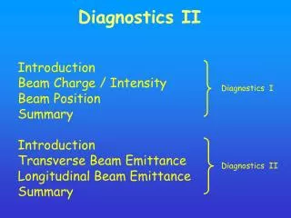
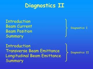
Diagnostics II. Introduction Beam Current Beam Position Summary Introduction Transverse Beam Emittance Longitudinal Beam Emittance Summary. Diagnostics I. Diagnostics II. Introduction. Reminder:. transformation of the phase space coordinates

Diagnostics II
E N D
Presentation Transcript
Diagnostics II Introduction Beam Current Beam Position Summary Introduction Transverse Beam Emittance Longitudinal Beam Emittance Summary Diagnostics I Diagnostics II
Introduction Reminder: transformation of the phase space coordinates (x,x’) of a single particle (from if) given in terms of the transport matrix, R Equivalently, and complementarily, the Twiss parameters (, , and ) obey The elements of the transfer matrix R are given generally by or if the initial and final observations points are the same, by the one-turn-map: where is the 1-turn phase advance: = 2Q
A third equivalent approach involves the beam matrix defined as in terms of Twiss parameters in terms of the moments of the beam distribution Here <x> and <x2> are the first and second moments of the beam distribution: where f(x) is the beam intensity distribution The transformation of the initial beam matrix beam,0to the desired observation point is where R is again the transfer matrix Neglecting the mean of the distribution (disregarding the static position offset of the core of the beam; i.e. <x>=0) : and the root-mean-square (rms) of the distribution is
Measurement of the Transverse Beam Emittance Method I: quadrupole scan Principle: with a well-centered beam, measure the beam size as a function of the quadrupole field strength Here Q is the transfer matrix of the quadrupole R is the transfer matrix between the quadrupole and the beam size detector With then with The (11)-element of the beam transfer matrix is found after algebra to be: o which is quadratic in the field strength, K
Measurement: measure beam size versus quadrupole field strength recall: o data: fitting function (parabolic): equating terms (drop subscripts ‘o’), solving for the beam matrix elements:
The emittance is given from the determinant of the beam matrix: With these 3 fit parameters (A,B, and C), the 3 Twiss parameters are also known: as a useful check, the beam-ellipse parameters should satisfy (xx-1)=2
Method II: fixed optics, measure beam size using multiple measurement devices Recall: the matrix used to transport the Twiss parameters: with fixed optics and multiple measurements of at different locations: simplify notation: x B o goal is to determine the vector o by minimizing the sum (least squares fit): with the symmetric nn covariance matrix, the least-squares solution is (the ‘hats’ show weighting: )
data: from the SLC injector linac once the components of o are known, graphical representation of results: note: coordinate axes are so norma- lized (design phase ellipse is a circle): lines show phase space coverage of wires: With methods I & II, the beam sizes may be measured using e.g. screens or wires
Transverse Beam Emittance – Screens principle: intercepting screen (eg. Al2O3Cr possibly with phosphorescent coating) inserted into beam path (usually 45 deg); image viewed by camera direct observation of x-y ( = 0) or y-( ≠ 0) distribution fluorescence – light emitted (t~10 ns) as excited atoms decay to ground state phosphorescence – light continues to emit (~ s) after exciting mechanism has ceased (i.e. oscilloscope “afterglow”) luminescence – combination of both processes R. Jung et al, “Single Pass Optical Profile Monitoring” ( DIPAC 2003) emittance measurement image is digitized, projected, fitted with Gaussian calibration: often grid lines directly etched onto screen or calibration holes drilled, either with known spacing issues spacial resolution (20-30 m) given by phosphor grain size and phosphor transparency temporal resolution – given by decay time radiation hardness of screen and camera dynamic range (saturation of screen) (courtesy P. Tenenbaum, 2003)
Transverse Beam Emittance – Transition Radiation (1) principle: when a charged particle crosses between two materials of different dielectric constant (e.g. between vacuum and a conductor), transition radiation is generated, temporal resolution is ~ 1 ps useful for high bunch repetition frequencies forward and backward transition radiation with foil at 45 degrees allowing for simple vacuum chamber geometry (courtesy K. Honkavaara, 2003) foil: Al, Be, Si, Si + Al coating, for example emittance measurement (as for screens): digitized and fitted image calibration: also with etched lines of known spacing issues: spacial resolution (<5 m) as introduced by the optics damage to radiator with small spot sizes (geometrical depth of field effect when imaging backward TR)
Transverse Beam Emittance – Transition Radiation (2) the SLAC-built OTR as installed in the extraction line of the ATF beam spot as measured with the OTR at the ATF at KEK (all figures courtesy M. Ross, 2003)
Transverse Beam Emittance – Wire Scanners (1) principle: precision stage with precision encoder propels shaft with wire support wires (e.g. C, Be, or W) scanned across beam (or beam across wire) interaction of beam with wire detected, for example with PMT wire mount used at the ATF (at KEK) with thin W wires and 5 m precision stepper-motors and encoders (courtesy H. Hayano, 2003) wire velocity: depends on desired interpoint spacing and on the bunch repetition frequency detection of beam with wire: 1. change in voltage on wire induced by secondary emission 2. hard Bremsstrahlung – forward directed s which are separated from beam via an applied magnetic field and converted to e+/e- in the vacuum chamber wall and detected with a Cerenkov counter or PMT (after conversion to s in front end of detector) 3. via detection at 90 deg (-rays) 4. using PMTs to detect scattering and electromagnetic showers (5. via change in tension of wire for beam-tail measurements) emittance measurement: as for screens (quad scan or 3-monitor method)
Transverse Beam Emittance – Wire Scanners (2) issues: different beam bunch for each data point no information on x-y coupling with 1 wire (need 3 wires at common location) dynamic range: saturation of detectors (PMTs) single-pulse beam heating wire thickness (adds in quadrature with beam size) higher-order modes (left) wire scanner chamber installed in the ATF (KEK) extraction line and (right) example wire scan (courtesy H. Hayano, 2003)
Transverse Beam Emittance – Synchrotron Radiation (1) principle: charged particles, when accelerated, emit synchrotron radiation measurements: imaging beam cross section • direct observation • angular spread depth of field effect in direct imaging (ref. A. Sabersky) phase space coordinates of the photon beam a = half-width of and l = distance to defining aperture measured beam parameterscorrespond to a projection of this phase space onto the horizontal axes photon beam phase space at distance l from source (for a 100 m beam at emission point)
Transverse Beam Emittance – Synchrotron Radiation (2) optics used at the SLC (damping rings) for imaging SR emitted in a dipole magnet (not to scale) gated camera synchro- nization using a standard TV camera intensifier of the gated camera used for fast (turn by turn) imaging of the radiation (from Xybion Corp.) (scrolling from emi removed using a line-locked TV camera for composite synchronization) key feature: gated high bias between photocathode and MCP
Transverse Beam Emittance – Synchrotron Radiation (3) (left) raw data showing turn-by-turn images at injection (average over 8 pulses) (bottom) digitized image in 3-D and projections together with Gaussian fits (bottom) originally, these studies aimed at measuring the transverse damping times, but were then extended to measure emittance mismatch and emittance of the injected beams …
Transverse Beam Emittance – Synchrotron Radiation (4) injection matching – using the definition of the mismatch parameter (M. Sands) (left) turn- by-turn beam size measured before (top) and after (bottom) injection matching; (right) spectrum of beam shape oscillations (FT of x2(t)) A1 = B = amplitude of DC peak A2=sqrt (B2-1) = amplitude of peak at 2Q with =A1/A2 B = 1/sqrt(1--2) beam emittance = A1 /(A22+1)
Transverse Beam Emittance – Laser Wire Scanners principle: laser wire provides a non-invasive and non-destructable target wire scanned across beam (or beam across wire) constituents: laser, optical transport line, interaction region and optics, detectors beam size measurements: forward scattered Compton s or lower-energy electrons after deflection by a magnetic field schematic of the laser wire system planned for use at PETRA and for the third generation synchrotron light source PETRA 3 (courtesy S. Schreiber, 2003) high power pulsed laser overview of the laser wire system at the ATF (courtesy H. Sakai, 2003) optical cavity pumped by CW laser (mirror reflectivity ~99+%)
laser-electron interaction point from the pioneering experiment at the SLC final focus (courtesy M. Ross, 2003) beam size measured at the laser wire experiment of the ATF (courtesy H. Sakai, 2003) (as with normal wires, the wire size must be taken into account) (here w0 is the 2 wire thickness) issues: waist of laser < beam size (in practice, waist size ~) background and background subtraction depth of focus large so that sensitivity of y on xe is minimized synchronization (for pulsed lasers)
Transverse Beam Emittance – Interferometric Monitor (T. Shintake) principle: laser provides a non-invasive and non-destructable target by splitting and recombining the laser light a standing wave (sw) is made the intercepting beam produces Compton-scattered photons of high density in the sw-peaks and of low density in the sw-valleys constituents: laser, optical transport line, interaction region and optics, detectors beam size measurements: scattered Compton ’s as a function of beam position (arbitrary phase) number of scattered photons <N>=A+Bcos(2kLx+) laser wave number (=2/L) fringe pattern of sw y x B/A 0 infinitely large beam B/A 1 infinitely small beam i.e. by scanning the beam position along the standing wave, the modulation depth of the observed photon spectrum gives information about the beam size
another conceptual illustration of the signal amplitude (courtesy T. Shintake, 2004) large beam size medium beam size small beam size
Measurements of small beam sizes at the FFTB (courtesy T. Shintake, 2004) y=1.95 m y=90 nm y=77 nm distribution of measurements
Issues for the single-pass interferometric monitor: Laser power imbalance (mirror “asymmetries”) Electron beam crossing angle (electron beam not parallel to the plane of the fringes) Longitudinal extent of the interference pattern (compare “hour-glass” effect) Laser alignment Spatial and temporal coherence of the laser (alignment distortions) Laser jitter
Beam Energy Spread In circular accelerators, the beam energy spread is usually very small (~10-4) In linear accelerators, the energy spread is determined to a large extent by the length of the bunch and its overlap with the sinusoidal accelerating voltage effective energy gain (left) and energy spread (right) for low (a) and high (b) current bunches illustrating optimum phasing of the rf structures for minimum energy spread Principle: the beam size as measured, e.g. with a screen or wire, is the convolution of the natural beam size , x,y and the energy spread =E/E: = sqrt ( 2 + []2) where is the dispersion function By proper selection of location (for a screen /wire), where is large, the beam energy spread can be directly measured
sketch of the layout of TTF I Single-bunch OTR images from TTF I obtained in a region of high dispersion (courtesy F. Stulle, 2003)
Bunch Length – Streak Cameras Principle: photons (generated e.g. by SR, OTR, or from an FEL) are converted to e-, which are accelerated and deflected using a time- synchronized, ramped HV electric field; e- signal is amplified with an MCP, converted to s (via a phosphor screen) and detected using an imager (e.g. CCD array), which converts the light into a voltage Principle of a streak camera (from M. Geitz, “Bunch Length Measurements”, DIPAC 99) Issues: energy spread of e- from the photocathode (time dispersion) chromatic effects (dt/dE()) in windows space charge effects following the photocathode
25 µs FS (every 4th turn) Streak camera images from the Pohang light source evidencing beam oscillations arising from the fast-ion instability (courtesy M. Kwon, 2000) 500 ns ( ~1/2 turn) FS
Bunch Length – Transverse Mode Cavities (1965: Miller,Tang, Koontz) Principle: use transverse mode deflecting cavity to “sweep”/kick the beam, which is then detected using standard profile monitors Principle of the TM11 transverse mode deflecting cavity introduce x-z correlation oriented to displace beam vertically while a horizontal bending magnet deflects the beam onto the screen y2 = A(Vrf-Vrf,min)2 = y02 z = A1/2E0rf/2R34 z expressed in terms of fit parameter, A (figures courtesy R. Akre, 2003)
Summary We reviewed multiple, equivalent methods for describing the transport of beam parameters between 2 points Two methods for measuring the transverse beam emittance were presented: the quadrupole scan – optics are varied, single measurement location the fixed optics method with at least three independent beam size measurements Methods for measuring the beam size were reviewed including screens transition radiation (conventional) wire scanners (direct imaging of) synchrotron radiation laser wires interferometric monitors The presented method for measuring the bunch energy spread used hardware as for the transverse beam size measurements, but required situation at a location where the dispersion is nonzero Bunch length measurements using streak cameras and transverse mode cavities were briefly reviewed