Download
1 / 29
290 likes | 385 Views
Midterm info . Wed Oct 12, 11:35-12:50 Place: TBA Covers: everything to next Monday Review sessions: M and T, 5 – 9, LC 211 Last year’s exam as an example (no answers). Business cycles and short run macro. Let’s review our voyage to date:. We have analyzed: Measuring economic activity

E N D
Midterm info • Wed Oct 12, 11:35-12:50 • Place: TBA • Covers: everything to next Monday • Review sessions: M and T, 5 – 9, LC 211 • Last year’s exam as an example (no answers)
Business cycles and short run macro
Let’s review our voyage to date: We have analyzed: • Measuring economic activity • Aggregate production functions and distribution • Classical AS and AD (flexible w and p) • Financial macro (including money) • Open-economy macro We now move on to • Business cycles, Keynesian economics, and the IS-MP model
The Great Divide Classical macro: - full employment - flexible wages and prices - Perfect competition and rational expectations - No business cycles (or “real” business cycles), and all unemployment is voluntary and efficient Keynesian macro: - Underutilized resources - Inflexible (or fixed) wages and prices - Imperfect competition and behavioral expectations - Yes, business cycles, with persistent slumps, involuntary unemployment, and macro waste.
Understanding business cycles Major elements of cycles • short-period (1-3 yr) erratic fluctuations in output • pro-cyclical movements of employment, profits, prices • counter-cyclical movements in unemployment • appearance of “involuntary” unemployment in recessions Historical trends • lower volatility of output, inflation over time (until 2008) • movement from stable prices to rising prices since WW II
Output gaps and business cycles Large GDP “gap”
Major approaches to business cycles • “Keynesian cross” (Econ 116): useful for intuition • AS-AD with p and Y (Econ 116): needs updating and will not use • IS-LM: from earlier era • IS-MP (Econ 122) • Mankiw’s dynamic model: mainstream modern Keynesian macro • Open-economy in short run: Mundell-Fleming: Very important approach to open economy
IS-MP model The major tool for showing the impact of monetary and fiscal polices, along with the effect of various shocks, in a short-run Keynesian situation. Key assumptions • Fixed prices (P=1 and π = 0) • Unemployed resources (Y < potential Y = Mankiw’s natural Y) • Closed economy (not essential and will be considered later) • Goods markets (IS) and financial markets (MP)
IS curve (expenditures) Basic idea: describes equilibrium in goods market Finds Y where planned I = planned S or planned expenditure = planned output Basic set of equations: • Y = C + I + G • C = a + b(Y-T) • T = T0 + τ Y [note assume income tax, τ = marginal tax rate] • I = I0 –dr [note i = r because fixed P] • G = G0
which gives the IS curve: Y =a - bT0 + G0 + I0 - dr 1 - b(1- τ) Y = μ [A0 - dr] where A0 = autonomous spending = a - bT0 + G0 + I0 μ = simple Keynesian multiplier = 1/[(1 - b(1- τ)] or in terms of solving for the interest rate: r = (A0 - Y/μ ) / d which we graph as the IS curve.
MP curve (monetary policy/financial markets) The MP curve represents equilibrium in financial markets. 1. Monetary Policy: Taylor Rule Begin with a monetary policy equation in the form of a “Taylor rule”: (TR) i = π + r* + b(π-π*) + cy r* is the equilibrium real interest rate, π inflation rate, π* is inflation target, y is log output gap [log(Y/Yp)], b and c are parameters.
MP curve (monetary policy/financial markets) The MP curve represents equilibrium in financial markets. 1. Monetary Policy: Taylor Rule Begin with a monetary policy equation in the form of a “Taylor rule”: (TR) i = π + r* + b(π-π*) + cy r* is the equilibrium real interest rate, π inflation rate, π* is inflation target, y is log output gap [log(Y/Yp)], b and c are parameters. 2. We will ignore inflation for now to simplify. Add that after have studied. So π = π* = 0 and we have financial market: (MP) r = r* + cy Later on, we will introduce inflation in the TR and MP.
Algebra of IS-MP Analysis • The analysis looks at simultaneous equilibrium in goods market and financial markets (Main St and Wall St). • The algebraic solution for equilibrium Ye is:***Ye = μ*A0 –μ* d r* where μ* = μ/(1 + μdc’) = multiplier with monetary policy. μ= simple multiplier > μ* ; A0 = autonomous spending = a - bT0 + G0 + I0 , Note impacts on output: Positive: G, I0, NX Negative: risk premium (and later inflation shock) *** There is a small technical issue in the algebra here. The Taylor rule has r as a function of y = ln(Y/Yp), whereas the IS is Y = f(r). We want to keep the Y in the equation because mulitpliers are dY/dG (see CBO figure below). And Taylor rule is in y (or sometimes u). So we need a change of variable. The best way is to use Taylor approximation (different Taylor), that ln(1+x)= x +o(x2) for x close to zero. So ln (1+Y/Yp-1) ≈ Y/Yp-1, so we substitute that into the MP. This will give new c’ = cYp. Analysis is identical.
IS-MP diagram r = real interest rate MP(r*) E re IS(G, T0, …) Ye Y = real output (GDP)
1. What are the effects of fiscal policy? • A fiscal policy is change in purchases (G) or in taxes (T0, t), holding monetary policy constant. • In normal times, because MP curve slopes upward, expenditure multiplier is reduced due to crowding out.
Fiscal policy in normal times r = real interest rate MP re IS’ IS Y = real output (GDP)
Multiplier Estimates by the CBO Congressional Budget Office, Estimated Impact of the ARRA, April 2010
US in current recession Policy has hit the “zero lower bound” three years ago.
Japan short-term interest rates, 1994-2010 Liquidity trap from 1996 to today: 15 years and counting.
Fiscal policy in liquidity trap r = real interest rate IS’ IS MP re Y = real output (GDP)
Can you see why macroeconomists emphasize the importance of fiscal policy in the current environment? “Our policy approach started with a major commitment to fiscal stimulus. Economists in recent years have become skeptical about discretionary fiscal policy and have regarded monetary policy as a better tool for short-term stabilization. Our judgment, however, was that in a liquidity trap-type scenario of zero interest rates, a dysfunctional financial system, and expectations of protracted contraction, the results of monetary policy were highly uncertain whereas fiscal policy was likely to be potent.” Lawrence Summers, July 19, 2009
Case 2. Monetary policy The MP curve represents monetary policy. That is, the central bank responds by lowering (raising) interest rates when output declines (rises). - somewhat confusing because Fed actually has discretion, so in a sense the Taylor rule is a forecast of how Fed will act given the economy and its objectives Note that cannot follow Taylor rule in liquidity trap (when nominal short risk-free rates are near zero).
Case 3. Monetarism Older approach that emphasized the supply of money. Very important tradition, particularly Friedman and Schwartz, A Monetary History of the United States. Deemphasized in Econ 122, but still important in many other views of macro (warning about dissensus)
Summary on IS-MP Model This is the workhorse model for analyzing short-run impacts of monetary and fiscal policy Key assumptions: - Fixed or rigid prices - Unemployed resources Now on to analysis of Great Depression in IS-MP framework.