Download

1 / 42
450 likes | 602 Views
Classical Planning via State-space search. COMP3431 Malcolm Ryan. What is planning?. Planning is an AI approach to control Deliberation about action Key ideas We have a model of the world Model describes states and actions Give the planner a goal and it outputs a plan

E N D
Classical Planningvia State-space search COMP3431 Malcolm Ryan
What is planning? Planning is an AI approach to control Deliberation about action Key ideas We have a model of the world Model describes states and actions Give the planner a goal and it outputs a plan Aim for domain independence Planning is search
Early History • GPS, Newell and Simon State-space search, means-ends analysis 1971 STRIPS, Fikes and Nilsson Introduced STRIPS notation for actions 1975 NOAH, Sacerdoti NONLIN, Tate First plan-space search planners 1989 ADL, Pednault An extension of the STRIPS action notation
Middle History 1991 SNLP, Soderland and Weld based on McAllester and Rosenblitt Plan-space search make easy 1994 UMCP, Erol and Nau Hierarchical Task Network planning 1995 SATPlan, Kautz and Selman Planning as a satisfiability problem 1995 GraphPlan, Blum and Furst A return to state-space search, using planning graphs. 1998 PDDL, McDermott et al Extending ADL to include… ?
Recent History 2000 TL-Plan, Bacchus and Kabanza Search control using temporal logic. 2003 MBP, Cimatti et al Planning as model checking. Planning with non-determinism. 2004 STAN and TIM, Long, Fox et al. Domain analysis. Exploiting symmetry.
Classical planning Classical planning is the name given to early planning systems (before about 1995) Most of these systems are based on the Fikes & Nilsson’s STRIPS notation for actions Includes both state-space and plan-space planning algorithms.
The Model Planning is performed based on a given model of the world. A model includes: • A set of states, S • A set of actions, A • A transition function, : S x A S
Restrictions on the Model • S is finite • is fully observable • is deterministic • is static (no external events) • S has a factored representation • Goals are restricted to reachability. • Plans are ordered sequences of actions • Actions have no duration • Planning is done offline
Example: Blocks World blue red green table
Example: Blocks World S = the set of all different configurations of the blocks A = the set of “move” actions describes the outcomes of actions move(red,blue,green)
States, actions and goals States, actions and goals are described in the language of symbolic logic. Predicates denote particular features of the world: Eg, in the blocks world: • on(block1, block2) • on_table(block) • clear(block)
Representing States States are described by conjunctions of ground predicates (possibly negated). on(blue, red) on(green, red) The closed world assumption (CWA) is employed to remove negative literals: on(blue, red) The state description is complete.
Representing Goals The goal is the specification of the task A goal is a usually conjunction of predicates: on(red, green) on_table(green) The CWA does not apply. So the above goal could be satisfied by: on(red, green) on_table(green) on(blue, red) clear(blue) …
Representing Actions Actions are described in terms of preconditions and effects. Preconditions are predicates that must be true before the action can be applied. Effects are predicates that are made true (or false) after the action has executed. Sets of similar actions can be expressed as a schema.
STRIPS operators An early but still widely used form of action description is as “STRIPS operators”. Three parts: Precondition A conjunction of predicates Add-list The set of predicates made true Delete-list The set of predicates made false
Blocks World Action Schema move(block, from, to) Pre: on(block, from), clear(block),clear(to) Add: on(block, to), clear(from) Del: on(block, from), clear(to)
Blocks World Actions Note that this action schema defines many actions: move(red, blue, green) move(red, green, blue) etc… We also need to define: move_to_table(block, from) move_from_table(block, to)
Representing Plans A plan is simply a sequence of actions.eg = move_from_table(red, blue), move(red, blue, green), move_to_table(red, green) We require that every action in the sequence is applicable, i.e. its precondition is true before it is executed.
Reasoning with STRIPS An action a is applicable in state s if its precondition is satisfied, ie: pre+(a) s pre-(a) s = The result of executing a in s is given by: (s,a) = (s – del(a)) add(a) This is called progressings through a
Progression example Taking the earlier example: s = on(red, blue), on_table(blue), clear(red), on_table(green), clear(green) a =move(red, blue, green) move(red,blue,green)
Progression example • Check action is applicable: on(red, blue), clear(red),clear(green) • Delete predicates from delete-list: on(red, blue), on_table(blue), clear(red), on_table(green), clear(green) • Add predicates from add-list: on_table(blue), clear(red), on_table(green), on(red, green),clear(blue)
Progression example 2 Consider instead the action a =move_from_table(blue, green) This has precondition: pre(a) = on_table(blue), clear(blue), clear(green) This action cannot be executed as clear(blue) is not in s. i.e. it is not applicable
Reasoning with STRIPS We can also regress states. If we want to achieve goal g, using action a, what needs to be true beforehand? An action a is relevant for g, if: g add(a) ≠ g del(a) = The result of regressing g through a is: -1(g,a) = (g – add(a)) pre(a)
Regression Example Take the goal: g = on(red, green), on_table(blue) Regress through action: a =move(red, blue, green) move(red,blue,green) ???
Regression Example • Check action is relevant: g add(a) = {on(red, green)} ≠ g del(a) = • Remove predicates from add list: on(red, green), on_table(blue) • Add preconditions: on_table(blue), on(red, blue), clear(red), clear(green)
Regression example 2 Consider instead the action a =move_to_table(red, blue) This has effects: add(a) = on_table(red), clear(blue) This action is not relevant as it does not achieve any of the goal predicates, ie: g add(a) =
Regression Example 3 Consider instead the goal g = clear(blue), clear(green) Now a = move(red, blue, green) achieves clear(blue) but is not relevant, as it conflicts with the goal: g del(a) = {clear(green)} ≠
Planning as state-space search Imagine a directed graph in which nodes represent states and edges represent actions. An edge joins two nodes if there is an action that takes you from one state to the other.
Graph of state space GOAL START
Forward/Backward chaining Planning can be done as forward or backward chaining. Forward chaining starts at the initial state and searches for a path to the goal using progression. Backward chaining starts at the goal and searches for a path to the initial state using regression.
Non-deterministic programming I will show planning algorithms using non-deterministic pseudocode The choose command will allow us to choose one of several paths to take. The fail command will indicate that a particular choice was unsuccessful.
Non-deterministic programming When we fail, we backtrack to the most recent choice with more options, and choose again Executing the code is then actually a search process Prolog is an example of such a language
Example SumToSeven() choosea {1,2,3,4,5} choose b {1,2,3,4,5} if (a + b == 7) then return {a,b} else fail
Example 2 SumToN(n) choosea {1,2,3,4,5} d = n – a if (d < 0) then fail else if (d == 0) then return {a} else return {a} SumToN(d)
Forward Search Forward-search(s, g) ifs satisfies gthen return empty plan applicable = {a | a is applicable in s} ifapplicable = then fail choose action a applicable s’ = (s,a) ’ = Forward-search(s’, g) return a.’
Backward Search Backward-search(s, g) ifs satisfies gthen return empty plan relevant = {a | a is relevant to g} ifrelevant = then fail choose action a relevant g’ = -1(g,a) ’ = Backward-search(s, g’) return ’.a
Pruning Search As in any search problem, an important element is to prune the search. Both of these algorithms have the potential to waste time exploring loops. A record should be kept of already visited states and actions that return to these states should be pruned. Backwards search can produce inconsistent goals (usually not pruned)
Instantiating Schema When using action schema often it is more efficient to instantiate schema variables on the fly, by unification, rather than generating and testing all instances.
Planning as Search Forward-search, backward-search and most other planning algorithms can be described in a similar structure: • Generate possible branches. • Prune those that are no good. • Select one remaining branch • Recurse
Bi-directional search We can apply bidirectional search to state-space planning, doing both progression from the start state and regression from the goal. Typical heuristic: • try both, then repeat whichever expansion took less time (as it is likely to again)
Heuristics for planning “cost to goal” = number of plan steps relaxed measure: number of plan steps disregarding delete effects h1(s,g) = max {h1(s,p) | p g} h1(s,p) = 0, if p s h1(s,p) = , if p is not in add(a) for any a h1(s,p) = min(1 + h1(s,pre(a)), p add(a)
Heuristics for planning h1 can be extended to h2 h3 … considering pairs of propositions, triplets, etc. All hk are admissible hk+1 dominates hk Computing hk is O(nk) with n propositions Generally k <= 2 is used