Download
1 / 45
500 likes | 752 Views
Financial analysis for vehicle program. Profit Analysis. Profit = Revenue – cost Where Revenue = selling price*number of vehicles sold Cost = investment cost + variable cost* number of vehicles produced Break even volume is the number of vehicles need to be sold so that there is no loss

E N D
Profit Analysis Profit = Revenue – cost Where Revenue = selling price*number of vehicles sold Cost = investment cost + variable cost* number of vehicles produced Break even volume is the number of vehicles need to be sold so that there is no loss Break even Volume = Investment cost/(selling price – variable cost)
Examples of Successful & Unsuccessful Programs Break even volume = 500,000,000/(22,000-17,000) = 100,000 vehicles
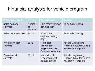
Your Calculations • Estimate selling price for your car from market survey • Estimate the number of vehicles that can be sold • Assume variable cost to be about X% of the selling price • Assume investment cost to be Y RM • Figure out break even volume and profit • Figure out a way to distribute investment and variable cost to systems Investment Cost Variable Cost Body Chassis Powertrain Climate Control Electrical Body Chassis Powertrain Climate Control Electrical
Weight Analysis Curb Weight : Weight of an assembled vehicle Gross Vehicle Weight (GVW) = Curb weight + passenger & cargo weight Corner weight = weight on each suspension Curb Weight Body Chassis Powertrain Climate Control Electrical
Vehicle-fixed Coordinate System • ISO (International Standards Organization) coordinate system • Defines directions with respect to the vehicle
Forces Acting on a Car, Truck or Motorcycle • Gravity • Tire normal forces (loads) • Tire shear forces (driving or braking) • Aerodynamic forces and moments • D’Alembert (acceleration) forces • Trailer hitch loads
Static Loads • Sitting statically on a level surface:
Longitudinal Dynamics • Dynamic load transfer • Acceleration limits • Braking limits • Aerodynamic forces/moments
Acceleration at Low Speed • Acceleration on a level surface with no aerodynamic reactions
Climbing a Grade • No aerodynamic or acceleration effects • For small angles: cosq = 1, sinq = q • q = Grade angle (in radians)
Aerodynamic Resistance Load Aerodynamic drag load DA = 0.5 ρ V2 CD A Where: CD = Aerodynamic drag Coefficient ρ = Air density A = Frontal Area of the vehicle
Tire Rolling Resistance Load Rolling resistance load Rx = Rxf + Rxr = fr Wf + fr Wr Where: fr = Rolling Resistance Coefficient Wr = Rear axle load Wf = Front axle load fr = 0.015 or 0.01*(1+ V/160) Where, V is vehicle speed in km/h
Powertrain Applications • Powertrain development • Architecture evaluation (FWD, RWD, 4WD) • Acceleration (0-100 kph, passing), top speed • Tuning (engine, torque converter, transmission matching) • Traction limits • Fuel economy
Powertrain Architecture • Traction-limited acceleration depends on loads on the drive wheels • I.e., Front wheel drive Rear wheel drive Four wheel drive
Powertrain Architecture • Components in a solid axle rear drive
Engine Dyno Performance • Steady speed; Wide Open Throttle (WOT)
Basic Acceleration Model • Simple acceleration model used by highway engineers • Acceleration is: • Proportional to power to weight ratio • Inversely proportional to speed
Example of Simple Model • Simple acceleration model used by highway engineers • It over-predicts performance with actual P/W ratios • Models are calibrated with effective P/W ratio Simulated Vehicle (250 kw, 1833 kg, with all losses) 100% Efficient 50% Efficient
Tractive Force Performance • Tractive force vs. speed: • Reflects engine torque curve • Depends on gear • Low (1st) gear • High tractive effort • Limited speed range • Higher gears expand the speed range but reduce tractive effort • Multiple gears approximate constant engine power • Continuously variable transmission (CVT) can follow constant engine power curve
Acceleration Performance (M+Mr) ax = T Ngf ηgf/r – Rx – DA – Rhx – W sinθ Where M = vehicle mass = W/g Mr = equivalent mass of rotating components ax = longitudinal acceleration T = Engine Toerque Ngf = combined ratio of transmission & final drive ηgf = combined efficiency of transmission & final drive Rx = Rolling resistance forces DA = Aerodynamic forces Rhx = Hitch forces θ = Inclination angle Mr = [(Ie+It)Ngf2 + IdNf2 + Iw]/r2 or Mr/M = 0.04Ngf+0.0025Ngf2 and Ie,It and Iw are engine, transmission, axle inertias
Top Speed Calculation T Ngf ηgf/r >= Rx + DA + Rhx + W sinθ If LHS > RHS, acceleration to higher speed is possible LHS = RHS corresponds to top speed in that gear
Powertrain System Design Aerodynamic Drag Rolling Resistance Climbing Grade Mass, Driveline Inertias Gear Inefficiencies Uncontrolled Variables Vehicle Acceleration Top Speed • Engine torque/power • Transmission Gear Ratios • Final Drive Gear Ratio • Torque Converter • Tire Size • Tire Traction Limit • Axle Roll Design Specifications
What is needed? • Procedure for calculating top speed and time to reach 100 km/h from 0 • Procedure to calculate top speed • spreadsheet
Torque Converter • Fluid coupling between engine and transmission • Stator: • Deflects return flow in direction of the impeller • Adds to torque of impeller • Turbine torque > engine torque • Zero output/input speed ratio is “stall” • Turbine input to transmission is typically two times engine torque
Brake Systems Applications • Proportioning evaluation • Weight variations (curb weight to GVWR) • High and low friction • Testing for regulatory compliance (FMVSS 105, 121..) • Stability in braking (e.g., split mu, FMVSS 135) • Evaluating effect of partial system failures
Wheel Lockup • Front wheel lockup will cause loss of ability to steer the vehicle • With rear wheel lockup, any yaw disturbance will initiate rotation of the vehicle making it unstable • Brake proportioning strategy should allow the front brakes to lock first if ABS is not provided
FMVSS Regulatory Requirements • A fully loaded passenger car with new brakes will stop from speeds 30/60 mph in distance with average deceleration of 17/18 ft/s^2 • A fully loaded passenger car with burnished brakes will stop from speeds 30/60/80 mph in distance with average deceleration of 17/19/18 ft/s^2 • A lightly loaded passenger car with burnished brakes will stop from speeds 60 mph in distance with average deceleration of 20 ft/s^2 • A fully and lightly loaded passenger car with brake failure will stop from speeds 60 mph in distance with average deceleration of 8.5 ft/s^2
Brake Proportioning Maximum brake force an axle can carry without locking μp(Wfs + Fxr*h/L) Front Axle Fxmf = ------------------------- 1 – μp*h/L μp(Wrs - Fxf*h/L) Rear Axle Fxmr = ------------------------- 1 + μp*h/L Where Fxf and Fxr are front and rear brake forces Wfs and Wrs are front and rear static weights μp is the peak brake coefficient h is the c.g. height L is the wheelbase
Brake Proportioning Brake Force Fx = Tb/r = G Pa/r Where Fx is front or rear brake force (N) Tb is front or rear brake torque (Nm) r is the tire rolling radius (m) G is front or rear brake gain (N.m/MPa) Pa is brake application pressure
What is needed • Explanation on how to draw braking limits on the chart • How to draw FMVSS requirement • How to draw applied brake force diagram • Brake pressure/brake torque relation • Brake proportion strategy graph
Performance Triangles Front Lockup Boundary 2000 1500 Front Brake Force Ideal Proportioning Proportioning Range 1000 Rear Lockup Boundary 500 0 0 500 1000 1500 2000 Rear Brake Force
Braking Efficiency Eb = Dx/μp Where Eb is the braking efficiency Dx is the actual deceleration μp is the braking coefficient
Braking Efficiency Calculation • Assume front and rear brake proportioning strategy such as • Pf = Pa and Pr = 0.8 Pa • Calculate front and rear axle brake forces • Fxf = 2Gf*Pf/r and Fxr = 2Gr*Pr/r • Calculate deceleration Dx • Dx = (Fxf+Fxr)/W • Calculate front and rear axle loads • Wf = Wfs + (h/L)(W/g)Dx • Wr = Wrs – (h/L)(W/g)Dx • Calculate braking coefficients μf and μr • μf = Fxf/Wf and μr = Fxr/Wr • Calculate braking efficiency Eb • Eb = Dx/ (higher of μf or μr) • 7. Increase Pa till desired level of Dx is reached
Brake System Design Aerodynamic Drag Rolling Resistance Mass, C.G., wheelbase Uncontrolled Variables Vehicle Deceleration Efficiency Locking Strategy • Brake Pressure • Brake Torque Gains • Brake Proportioning • Tire Size • Tire Friction Limit Design Specifications
Energy/Power Absorption Energy and power absorbed by the brake system during braking E = MV2/2 P = MV2/(2ts) Where M is the mass of the vehicle V is the initial speed ts is the time to stop