Download
1 / 27
270 likes | 396 Views
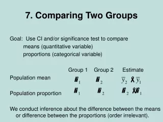
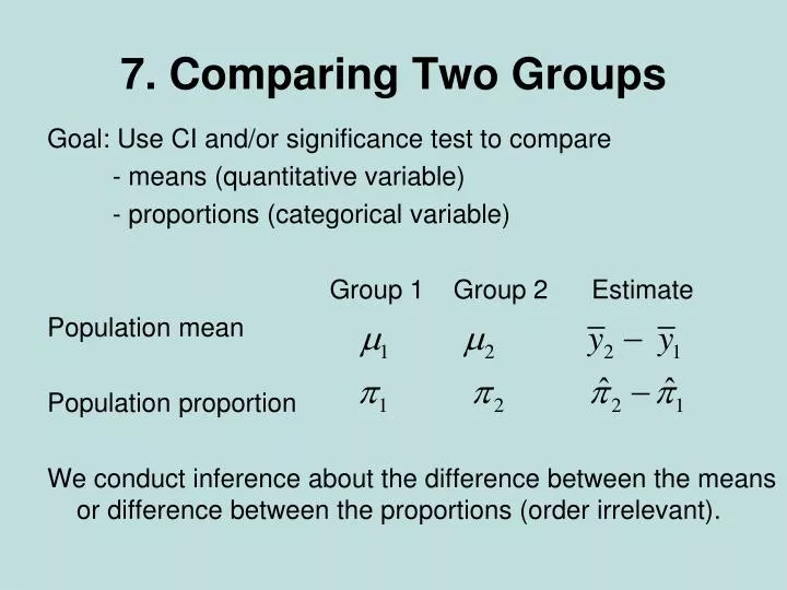
7. Comparing Two Groups. Goal: Use CI and/or significance test to compare - means (quantitative variable) - proportions (categorical variable) Group 1 Group 2 Estimate Population mean Population proportion

E N D
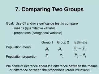
7. Comparing Two Groups Goal: Use CI and/or significance test to compare - means (quantitative variable) - proportions (categorical variable) Group 1 Group 2 Estimate Population mean Population proportion We conduct inference about the difference between the means or difference between the proportions (order irrelevant).
Example: Does cell phone use while driving impair reaction times? • Purpose of study: Analyze whether (conceptual) population mean response time differs significantly for the two groups, and if so, by how much. • Data in millisec. • Cell-phone group: • = 585.2 • s1 = 89.6 • Control group: • = 533.7 • s2 = 65.3.
se for difference between two estimates (independent samples) • The sampling distribution of the difference between two estimates is approximately normal (large n1 and n2)and has estimated Example: Data on “Response times” has 32 using cell phone with sample mean 585.2, s = 89.6 32 in control group with sample mean 533.7, s = 65.3 What is se for difference between sample means of 585.2 – 533.7 = 51.4?
(Note this is larger than each separate se. Why?) So, the estimated difference of 51.4 has a margin of error of about 2(19.6) = 39.2 (more precise details later using t distribution) 95% CI for m1– m2 is about 51.4 ± 39.2, or (12, 91). Interpretation: We are 95% confident that population mean m1 for cell phone group is between 12 milliseconds higher and 91 milliseconds higher than population mean m2 for control group. (In practice, good idea to re-do analysis without outlier, to check its influence. What do you think would happen?)
Quantitative Responses: Comparing Means • Parameter: m2 - m1 • Estimator: • Estimated standard error: • Sampling dist.: Approximately normal (large n’s, by CLT) • CI for independent random samples from two normal population distributions has form • Formula for df for t-score is complex (later). If both sample sizes are at least 30, can just use z-score
Example: GSS data on “number of close friends” Use gender as the explanatory variable: 486 females with mean 8.3, s = 15.6 354 males with mean 8.9, s = 15.5 Estimated difference of 8.9 – 8.3 = 0.6 has a margin of error of 1.96(1.09) = 2.1, and 95% CI is 0.6 ± 2.1, or (-1.5, 2.7).
We can be 95% confident that the population mean number of close friends for males is between 1.5 less and 2.7 more than population mean number of close friends for females. • Order is arbitrary. 95% CI comparing means for females – males is (-2.7, 1.5) • When CI contains 0, it is plausible that the difference is 0 in the population (i.e., population means equal) • Here, normal population assumption clearly violated. For large n’s, no problem because of CLT, and for small n’s the method is robust. (But, means may not be relevant for very highly skewed data.) • Alternatively could do significance test to find strength of evidence about whether population means differ.
Significance Tests for m2 - m1 • Typically we wish to test whether the two population means differ (null hypothesis being no difference, “no effect”). • H0: m2 - m1 = 0 (m1 = m2) • Ha: m2 - m1 0 (m1 m2) • Test Statistic:
Test statistic has usual form of (estimate of parameter – H0 value)/standard error. • P-value: 2-tail probability from t distribution • For 1-sided test (such as Ha: m2 - m1 > 0), P-value= one-tail probability from t distribution (but, not robust) • Interpretation of P-value and conclusion using -level same as in one-sample methods ex. Suppose P-value = 0.58. Then, under supposition that null hypothesis true, probability = 0.58 of getting data like observed or even “more extreme,” where “more extreme” determined by Ha
Example: Comparing female and male mean number of close friends, H0: m1 = m2 Ha: m1m2 Difference between sample means = 8.9 – 8.3 = 0.6 se = 1.09 (same as in CI calculation) Test statistic t = 0.6/1.09 = 0.55 P-value = 2(0.29) = 0.58 (using standard normal table) If H0 true of equal population means, would not be unusual to get samples such as observed. For = 0.05 = P(Type I error), not enough evidence to reject H0. (Plausible that population means are identical.) For Ha: m1 < m2 (i.e., m2 - m1 > 0), P-value = 0.29 ForHa: m1 > m2 (i.e., m2 - m1 < 0), P-value = 1 – 0.29 = 0.71
Equivalence of CI and Significance Test “H0: m1 = m2 rejected (not rejected) at = 0.05 level in favor ofHa: m1m2” is equivalent to “95% CI for m1 - m2 does not contain 0 (contains 0)” Example: P-value = 0.58, so “We do not reject H0 of equal population means at 0.05 level” 95% CI of (-1.5, 2.7) contains 0. (For other than 0.05, corresponds to 100(1 - )% confidence)
Alternative inference comparing means assumes equal population standard deviations • We will not consider formulas for this approach here (in Sec. 7.5 of text), as it’s a special case of “analysis of variance” methods studied later in Chapter 12. This CI and test uses t distribution with df = n1 + n2 - 2 • We will see how software displays this approach and the one we’ve used that does not assume equal population standard deviations.
Example: Exercise 7.30, p. 213. Improvement scores for therapy A: 10, 20, 30 therapy B: 30, 45, 45 A: mean = 20, s1 = 10 B: mean = 40, s2 = 8.66 Data file, which we input into SPSS and analyze Subject Therapy Improvement 1 A 10 2 A 20 3 A 30 4 B 30 5 B 45 6 B 45
Test of H0: m1 = m2 Ha: m1m2 Test statistic t = (40 – 20)/7.64 = 2.62 When df = 4, P-value = 2(0.0294) = 0.059. For one-sided Ha: m1< m2 (i.e., predict before study that therapy B is better), P-value = 0.029 With = 0.05, insufficient evidence to reject null for two-sided Ha, but can reject null for one-sided Ha and conclude therapy B better. (but remember, must choose Ha ahead of time!)
How does software get df for “unequal variance” method? • When allow s12 s22 recall that • The “adjusted” degrees of freedom for the t distribution approximation is (Welch-Satterthwaite approximation) :
Some comments about comparing means • If data show potentially large differences in variability (say, the larger s being at least double the smaller s), safer to use the “unequal variances” method • One-sidedt tests not robust against severe violations of normal population assumption, when n is small. Better then to use “nonparametric” methods (which do not assume a particular form of population distribution) for one-sided inference; see text Sec. 7.7. • CI more informative than test, showing whether plausible values are near or far from H0.
Effect Size • When groups have similar variability, a summary measure of effect size is • Example: The therapies had sample means of 20 for A and 40 for B and standard deviations of 10 and 8.66. If common standard deviation in each group is estimated to be s = 9.35 (say), then effect size = (40 – 20)/9.35 = 2.1. Mean for therapy B estimated to be about two standard deviations larger than the mean for therapy A. This is a large effect.
This effect size measure is sometimes called “Cohen’s d.” He consideredd = 0.2 = weak, d = 0.5 = medium, d > 0.8 large.Example: Which study showed the largest effect?
Comparing Means with Dependent Samples • Setting: Each sample has the same subjects (as in longitudinal studies or crossover studies) or matched pairs of subjects • Then, it is not true that for comparing two statistics, • Must allow for “correlation” between estimates (Why?) • Data: yi = difference in scores for subject (pair) i • Treat data as single sample of difference scores, with sample mean and sample standard deviation sdandparameter md = population mean difference score. • In fact, md = m2– m1
Example: Cell-phone study also had experiment with same subjects in each group (data on p. 194 of text) For this “matched-pairs” design, data file has the form Subject Cell_no Cell_yes 1 604 636 2 556 623 3 540 615 … (for 32 subjects) Sample means are 534.6 milliseconds without cell phone 585.2 milliseconds, using cell phone
We reduce the 32 observations to 32 difference scores, 636 – 604 = 32 623 – 556 = 67 615 – 540 = 75 …. and analyze them with standard methods for a single sample = 50.6 = 585.2 – 534.6, sd = 52.5 = std dev of 32, 67, 75 … For a 95% CI, df = n – 1 = 31, t-score = 2.04 We get 50.6 ± 2.04(9.28), or (31.7, 69.5)
We can be 95% confident that the population mean using a cell phone is between 31.7 and 69.5 milliseconds higher than without cell phone. • For testing H0 : µd = 0 against Ha : µd 0, the test statistic is t = ( - 0)/se = 50.6/9.28 = 5.46, df = 31, Two-sided P-value = 0.0000058, so there is extremely strong evidence against the null hypothesis of no difference between the population means.
In class, we will use SPSS to • Run the dependent-samples t analyses • Plot cell_yes against cell_no and observe a strong positive correlation (0.814), which illustrates how an analysis that ignores the dependence between the observations would be inappropriate. • Note that one subject (number 28) is an outlier (unusually high) on both variables • With outlier deleted, SPSS tell us that t = 5.26, df = 30 for comparing means (P = 0.00001) for comparing means, 95% CI of (29.1, 66.0). The previous results were not influenced greatly by the outlier.
SPSS output for original dependent-samples t analysis (including the outlier)
Some comments • Dependent samples have advantages of (1) controlling sources of potential bias (e.g., balancing samples on variables that could affect the response), (2) having a smaller se for the difference of means, when the pairwise responses are highly positively correlated (in which case, the difference scores show less variability than the separate samples) • With dependent samples, why can’t we use the se formula for independent samples?
Ex. (artificial, but makes the point) Weights before and after anorexia therapy Subject Before After Difference 1 115 122 7 2 91 98 7 3 100 107 7 4 132 139 7 … Lots of variability within each group of observations, but no variability for the difference scores (so, actual se is much smaller than independent samples formula suggests) If you plot x = before against y = after, what do you see?