Download
1 / 64
660 likes | 1.22k Views
Pipe System Design. CE154 - Hydraulic Design Lecture 7. Pump System. Pump Terminology. Pump head (dynamic head) – H Pump discharge – Q Pump speed – n Pump power – P. Centrifugal Pump. Rotary Pump. Reciprocating Pump. Pump Terminology. Power P. Motor efficiency m. Q, H. Pump

E N D
Pipe System Design CE154 - Hydraulic Design Lecture 7 CE154
Pump System CE154
Pump Terminology • Pump head (dynamic head) – H • Pump discharge – Q • Pump speed – n • Pump power – P CE154
Centrifugal Pump CE154
Rotary Pump CE154
Reciprocating Pump CE154
Pump Terminology • Power P Motor efficiency m Q, H Pump Efficiency p CE154
Pump Terminology • Pump Output (Water) Power (Q in gpm, H in ft, s is specific gravity and dimensionless, and P in horsepower) • Pump Input (Brake) Power CE154
Pump Terminology • Electric Motor Power • Typically motor efficiency is approximately 98% CE154
Pump Terminology • Single or Double suction pump • Single or multiple stage pump CE154
Pump Specific Speed • Q is gpm per suction, n is rpm, H is ft per stage CE154
Pump Performance • Variable-Speed pumps – may be desirable when different operating modes require different pump head or flow • Homologous lawsQ1/Q2 = n1/n2H1/H2 = (n1/n2)2P1/P2 = (n1/n2)3 CE154
Pump Performance Curves CE154
Pump Terminology • Static Lift – elevation difference between pump centerline and the suction water surface. If the pump is higher, static lift is positive. If pump is lower, static lift is negative. • Static Discharge – elevation difference between the pump centerline and the end discharge point. If pump is higher, static discharge is negative. • Total Static Head – sum of static lift and static discharge. CE154
Pump Terminology • Shutoff Head – head at 0 flow • Operating point – the point where the pump curve and the system curve intersect. A system curve is a curve describing the head-flow relationship of the pipeline system. CE154
System Curve friction losses CE154
Operating Point CE154
Pump Terminology • Net positive suction head (NPSH)- to ensure that water does not vaporize at the pump impeller tip- NPSH available = available suction head + atmospheric pressure – vapor pressure – suction head loss = determined by local condition- NPSH required = characteristic of and provided by pump curve CE154
Atmospheric Pressure • At mean sea level, 1 atomospheric pressure = 14.69 psia = 1.03 kg/cm2 = 760 mm Hg CE154
Vapor pressure • Vapor pressure of water at atmospheric pressure CE154
Pipe System Design • Determine system curve- identify all loss-incurring elements including friction, transitions, fittings, valves and other special equipment in the system (use Darcy-Weisbach equation to compute friction loss) - identify suction and discharge conditions CE154
Design Scenario – Ex. 8-1 • Need to deliver water from Santa Teresa Water Treatment Plant at elevation 300 ft to Cisco Power Plant at elevation 330 ft. The maximum flow demand is 200 cfs. Design pipe size and regulating devices for operation. • Basic design approach- consider steady-state, governing case- design pipe size and control equipment- check transient condition to verify pipe pressure class CE154
Example 8-1 • Prepare a list of available design data:- Design discharge 200 cfs- Suction water elevation El. 300 ft North Am. Vertical Datum (NAVD88 )- Discharge water elevation El. 330 ft NAVD88 • Prepare a list of data requirements:- Topographic maps to route pipeline- Right of way maps- Utility and road crossing maps CE154
Example 8-1 - Select a pump station site to set preliminary pump elevation: -- assume 2 Pumps set at El. 290 ft -- station design includes 40 ft of pipeline, 4 isolation valves and 2 pump discharge valves - No other information on discharge site is needed (for hydraulic design), other than the maximum tank level at 330 ft. CE154
Example 8-1 3. Assume that we have selected a route that results in a pipeline 8.0 miles long, and the fittings include - 80 bends of 90, - 25 bends of 45, - 10 butterfly valves for isolation 4. Determine pipe diameter- rule of thumb – maintain operating velocity at 6-8 ft/sec (h V2, consider economic analysis later) CE154
Example 8-1 Pipe Sizing • Design maximum discharge Q = 200 cfsassume V = 8 ft/sec A = 200/8 = 25 ft2 D = 5.64 ft = 67.7 inches Say D = 72 inch – why? A = 28.27 ft2 V = 7.1 ft/sec • Next, determine pipe material. For this size, steel and reinforced concrete pipes are available. Say RCP. CE154
Example 8-1 CE154
Example 8-1 Friction loss • From roughness chart, for 72” concrete pipes, in the mid roughness range, i.e., not new but not seriously corroded, e/D = 0.0005 f=0.017 • From equation for turbulent rough flows, • f = 0.017 O.K. CE154
Example 8-1 Friction loss • When the pipe is significantly corroded, the chart shows that e/D = 0.0017 and f=0.023 • When new pipe, the chart shows e/D = 0.000165 and f=0.0135 • Use the mid roughness values for design, and use the new pipe and rough pipe values to check the system design to ensure operability. CE154
Example 8-1 Friction loss • Compute friction loss:h = f L/D V2/2g = 0.017 x 8 x 5280 / 6 x V2/2g = 119.7 V2/2g = 119.7 x (7.1)2/2/32.2 = 93.7 ft • Compute minor losses:Size the butterfly valves: Use Val Matic valve data CE154
Example 8-1 Valve data • Val Matic butterfly valve data CE154
Example 8-1 Valve sizing • Q=Cv(P)1/2 • Q = 200 cfs x 448.8 gpm/cfs = 89760 gpm • Considerations:- use the smallest size of valve that can pass the design flow with acceptable head losses CE154
Example 8-1 Valve loss • For this example, let’s try 72” valves. • At 266500 gpm, the valve incurs 1 psi of loss.In terms of • Q = 266500 gpm = 593.8 cfsA = 28.27 ft2, V = 21.0 fps, h = 1 psi = 2.31 ft, kv = 0.337 • At 200 cfs, V=7.1 fps, h = 0.26 ft per valve CE154
Example 8-1 Minor loss • Compute 90 bend losses:Assume r/D=2, from Slide 34 of last lecture, kb90 = 0.19There are 80 bends at 90. • Compute 45 bend losses (25 of them):Assume r/D=2, kb45 = 0.1 (Crane TP410). There are 25 bends at 45 CE154
minor loss Reference • This web link provides a few pages from the Crane Co. technical paper 410 (selling for $35 at Crane Co.) for calculating minor losses http://www.lightmypump.com/help16.html CE154
Example 8-1 System head loss • Compute total head loss: • Since we have suction piping as well, compute loss in the suction pipe CE154
Example 8-1 Pipe sizing • Assume the pump station has 2 pumps. To have the same velocity in the pipes, the pump discharge and suction pipe diameter is 54”. • Additionally, 1 pipe bifurcation and 1 combining to contribute to minor losses CE154
Example 8-1 Pump Station Loss • Losses at pump station: • f = 0.0175 from Slide 32, Lecture 8 • hf = (0.0175 x 40 / 4.5)V542/2g = 0.16V542/2g • Bifurcation loss: kbi = 0.3 V542/2g • Combining loss: kcm = 0.5 V542/2g • Valve loss: kv = (0.337 x 2 +3.0) V542/2g • Total loss = 4.63 V542/2g CE154
Example 8-1 – System Schematics El. 330 ft Hp El. 300 ft El. 290 ft CE154
Example 8-1 – System Curve • Total static headHst = 330-300 = 30 ft • Lossespump station loss + pipeline loss= 4.63 V542/2g + 140.8 V722/2g= 4.63 Q542/(2gA542) + 140.8 Q722/(2gA722)= 4.63 Q722/(8gA542) + 140.8Q722/51483.8)= 4.63Q2/65159.2 + 140.8Q2/51483.8= (0.000071 + 0.002734)Q2= 0.002805Q2 CE154
Example 8-1 – System Curve • System CurveH = 30 + 0.002805 Q2 CE154
Example 8-1 – System Curve • The Q in system curve is the total flow • Since we have 2 pumps, each pump puts out half of the total Q • In this case, need to construct the 2-parallel-operating pump curve by doubling the flows • Plot the system curve over the pump curve to determine the pump operation point CE154
8-1 Pump Operating Point • Select 17.57” impeller CE154
Ex. 8-1 Pump operating point • For new and old pipe conditions, revise system curves and determine if the pump can operate at these limits. In new pipes, pump may run-out (fall off the far end of the pump curve), or not meeting the higher NPSH requirement. • In really old pipes, pump may not be able to deliver the required flow rate. CE154
Ex. 8-1 New Pipe Operation • In this case, new pipe f=0.0135 instead of 0.017. Friction loss coefficient becomes 116.2 instead of 140.8. System curves becomes H = 30 + 0.002326Q2 CE154
Ex. 8-1 Pump Suction Design • Verify NPSHA meets NPSHR • Assume average temperature of 68F, • hatm = 14.53 psia, interpolated from Table on Slide 18 • hv = 0.339 psia • hs = 300-290 = 10 ft • hs = 4.63 V542/2g = 4.63 (6.29)2/64.4 = 2.84 ft • NPSHA = (14.53-0.339)x2.31 + 10 – 2.84 = 39.9 ft • NPSHR = 7 ft from pump curve OK CE154