Download
1 / 57
570 likes | 594 Views
Dive into the life and work of Jerzy Neyman, a pioneering statistician, and explore stochastic models, population dynamics, and his impact on various fields. Learn about Neyman's groundbreaking research and applications in agriculture, astronomy, and more.

E N D
Dynamic Indeterminism in Science David R. Brillinger Statistics Department University of California, Berkeley www.stat.berkeley.edu/~brill brill@stat.berkeley.edu
1. INTRODUCTION I. Neyman II. Stochastics III. Population dynamics IV. Moving particles V. Discussion A succession of examples, some JN’s, some DRB + collaborators’
I. NEYMAN 1894 Born, Bendery, Monrovia 1916 Candidate in Mathematics, U. of Kharkov 1917-1921 Lecturer, Institute of Technology, Kharkov 1921-1923 Statistician, Agricultural Research Inst, Bydgoszcz, Poland 1923 Ph.D. (Mathematics), University of Warsaw 1923-1934 Lecturer, University of Warsaw Head, Biometric Laboratory, NenckiInst. 1934-1938 Lecturer, then Reader, University College
1938 Professor of Mathematics, UC Berkeley • Statistics Department, UCB • 1961 Professor Emeritus, UCB • 1981 Died, Oakland, California
2. THE MAN. Polish ancestry and very Polish. “His devotion to Poland and its culture and traditions was very marked, and when his influence on statistics and statisticians had become world wide it was fashionable ... to say that `we have all learned to speak statistics with a Polish accent' …” D.G. Kendall (1982) Twinkle in the eye - coat Own money for visitors and students Drinks at Faculty Club “To the ladies present, and …” Soccer “I was one of the forwards, not on the center, …, but on the left. … I could run fast.”
Many, many visitors to Berkeley “He seemed to know personally all the statisticians of the world.” T. L. Page (1982) Strong social conscience “this is in connection with the current developments in the South, including the arrests of large numbers of youngsters, their suspension or dismissal from schools, the tricks used to prevent Negroes from voting, …” Neyman and others (1963)
3. NEYMAN’S WORK. “… the delight I experience in trying to fathom the chance mechanisms of phenomena in the empirical world.” Neyman(1970) 215 research papers From 1948, 55 out of 140 with E.L.Scott
Special influences. K. Pearson (The Grammar of Science), R. A. Fisher (Statistical Methods for Research Workers) “… there is not the slightest doubt that his (RAF’s) many remarkable achievements had a profound influence on my own thinking and work.” Neyman (1967) Applied at the start (agriculture) and at the end (Using Our Discipline to Enhance Human Welfare)
Applications. Agriculture, astronomy, cancer, entomology, oceanography, public health, weather modification, … Theory. CIs, testing, sampling, optimality, C(α), BAN, …
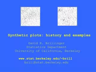
How were models validated? Observed and expected Formal tests with broad alternatives Chi-squared “appears reasonable”, “satisfactory fit”, … “… the method of synthetic photographic plates” Neyman, Scott, Shane (1952) One simulates realizations of a fitted model
Synthetic Photographic plate
Discovered variability beyond elementary clustering “When the calculated scheme of distribution was compared with the actual …, it became apparent that the simple mechanism could not produce a distribution resembling the one we see.” Neyman and Scott (1956)
II. STOCHASTICS “The essence of dynamic indeterminism in science consists in an effort to invent a hypothetical chance mechanism, called a 'stochastic model', operating on various clearly defined hypothetical entities, such that the resulting frequencies of various possible outcomes correspond approximately to those actually observed.” Neyman(1960) “… stochastic is used as a synonym of indeterministic.” Neyman and Scott (1959)
4. RANDOM PROCESSES. Time series. Chapter in Neyman (1938) Markov. “Markov is when the probability of going - let's say - between today and tomorrow, whatever, depends only on where you are today. That's Markovian. If it depends on something that happened yesterday, or before yesterday, that is a generalization of Markovian.” Neyman in Reid (1998) States of health, Fix and Neyman (1951)
State space model. Vector contains basic information concerning evolution Can incorporate background knowledge Can make situation Markov Evolution/dynamic equation Measurement equation
III. POPULATION DYNAMICS 6. SARDINES. In 1940s Neyman called upon to study the declining sardine catches along the West Coast.
“Certain publications dealing with the survival rates of the sardines begin with the assumption that both the natural death rate and the fishing mortality are independent of the age of the sardines, …” Neyman(1948) Na,t: fish aged a available year t N(t) = [Na,t]: state vector na,t: expected number caught qa: natural mortality age a Qt: fishing mortality year t Model: Na+1,t+1 = Na,t(1-qa)(1-Qt) H0: qb = qb+1 = … = qa , a > b
“… the death rate has a component which increases with the increase in age of the sardines. It may be presumed that this component is due to natural causes.” Neyman(1948)
Tables of fitted and observed. “While in certain instances the differences between Tables IV and VII are considerable, it will be recognized that the general character of variation in the figures of both tables is essentially similar.” (ibid) How to study further? HA? Neyman et al (1952), astronomy EDA: plot |X-Y| versus (X+Y)/2
7. Lucilia cuprina. Guckenheimer, Gutttorp, Oster & DRB in late 70s studied A. J. Nicholson’s blowfly data.
Obtaining the data Population maintained with limited food for 2 years Started with pulse Counts of eggs, emerging, deaths every other day Life stages egg: .5 – 1.0 day larva: 5-10 days pupa: 6-8 days adult: 1-35 days
Question: Dynamical system leading to chaos? State space setup. Na,t: number aged a on occasion t Et: number emerging = N0,t Nt: state vector = [Na,t] Nt: number of adults = 1’Nt Dt: number dying = Nt-1 + Et – Nt qa,t: Prob{individual aged a dies aged a | history} Dt | history fluctuates about Σaqa,tNa,t
Age and density dependent model, qa,t = 1 – (1-αa)(1-βNt)(1-γNt-1) αa: dies | age a βNt: dies | Nt adults γNt-1: dies |Nt-1, preceding time NLS, weights Nt2
Blowfly conclusions. Death rate age/density dependent Nonlinear dynamic system, chaos possible “Nicholson was using the flies as a computer.” P.A.P. Moran (late 70s)
IV MOVING PARTICLES 8. CLOUD SEEDING. JN started work in early 50s California, Arizona, Switzerland Emphasized importance of randomization Hail suppression experiment Grossversuch III, Ticino Suitable days (thunderstorm forecast) Silver iodide seeding from ground generators
DRB (1995) Particles born at Ticino at times σj Point process, {σj}, has rate pM(t) t, time of day Travel times independent, density f(.) Particles arrive at Zurich at rate pN(t) pN(t) = ∫ pM(t-u)f(u)du
μR: mean rain per particle X: cumulative process of rain pX(t): rate of rainfall pX(t) = μR∫ pM(t-u)f(u) du E{X(t)} = ∫0t pX(v)dv α: rate of unrelated rainfall
Running mean [X(t+1)-X(t-2)]/3 pM(t) = C, A < t < B Regression function. α + C0μR [∫ab F(u)du- ∫cd F(u)du] a = t-2-A, b = t+1-A, c = t-2-B, d = t+1-B Travel velocities, gamma OLS, weights 53 and 38
Approximate 95% CI for travel time. 5.50 ± 1.96(.76) Seeding started at 7.5 hr CI for T, arrival time of effect 13.0 ± 1.5 hr
12. Equations of motion. DEs. Newtonian motion Described by potential function, H Planar case, location r = (x,y)’, time t dr(t) = v(t)dt dv(t) = - βv(t)dt – β H(r(t),t)dt v: velocity β: coefficient of friction dr = - H(r,t)dt = μ(r,t)dt, β >> 0 Advantage of H - modelling
SDEs. dr(t) = μ(r(t),t)dt + σ(r(t),dt)dB(t) μ: drift (2-)vector σ: diffusion (2 by 2-)matrix {B(t)}: bivariate Brownian (Continuous Gaussian random walk) SDE benefits, conceptualization, extension
Solution/approximation. (r(ti+1)-r(ti))/(ti+1-ti) = μ(r(ti),ti) + σZi+1/√(ti+1-ti) Euler scheme Approximate likelihood
14. ELK. DRB et al(2001 - 2004) Starkey Reserve, Oregon Can elk, deer, cows, humans coexist? NE pasture
Rocky Mountain elk (Cervus elaphus) 8 animals, control days, Δt = 2hr Part A. Model. dr = μ(r)dt + σdB(t) μ smooth - geography Nonparametric fit Estimate of μ(r):velocity field
Synthetic path. Boundary (NZ fence) dr(t)= μ(r(t),t)dt + σ(r(t),dt)dB(t) +dA(r(t),t) A, support on boundary, keeps particle in What is the behavior at the fence?
Part B. Experiment with explanatory Same 8 animals ATV days, Δt = 5min