Download
1 / 25
250 likes | 378 Views
GG 313 Lecture 7. Chapter 2: Hypothesis Testing Sept. 13, 2005. CRUISE. Non- required planning meeting for all involved This Friday 1:30 PM, POST 703. Let’s go over the homework and finish up the last of Chapter 2 first. Homework being returned:

E N D
GG 313 Lecture 7 Chapter 2: Hypothesis Testing Sept. 13, 2005
CRUISE Non- required planning meeting for all involved This Friday 1:30 PM, POST 703
Let’s go over the homework and finish up the last of Chapter 2 first. Homework being returned: • Do your calculations in Matlab or Excel and DOCUMENT them. • You should be able to determine what a reasonable answeris. If your answer isn’t reasonable, its probable that it’s wrong! I take off points for unreasonable answers.
Today’s homework: 1) Hawaiian data: What did you get for a correlation coefficient? Are age and distance correlated? (We’ll come back to these data set later.) 2) chromium: You can use the functions in Matlab, but to be sure you understand them, I strongly suggest that you try your own functions and compare the two. Any bad points? Is nickel correlated? 3) Generate the plots
Inferences about Population Mean We estimate the mean of a population by calculating the mean of our sample. Knowing from the central limit theorem that the sample mean estimate should be normally distributed about the population mean, we can get some idea of the precision of our estimate of the population mean. Here’s one place where I found Paul’s notes near impossible to understand. Read his notes, and try the following explanation.
If we took many trials, our sample mean, x, would have a normal distribution about the population mean, µ. From earlier, the standard deviation of the sample mean is equal to the population standard deviation divided by the √n: (see Eqn. 1.101) Thus, the deviation of our sample mean from the population mean has a normal distribution defined by a mean of 0=x-µ, and a variance of 2/n. Changing to normalized coordinates, We have used s as an approximation to . This ASSUMES that n is LARGE (>30).
We want a zi that will give us appropriate confidence limits for our estimate of the mean. Zi=2, for example is 2 standard deviations from the mean, with a probability that the estimate will be within zi=±2 of 95%, thus, this is the 95% confidence interval. We want to solve for the xi appropriate for that zi. If we wanted a 97% confidence interval, we would use zi=3, and so forth. Paul calls this special value of zi z/2, and the special value of xi he calls E.
The probability that x is greater than the confidence interval z/2 is . When n~30 or more, and the population is infinite, we can substitute the sample standard deviation, sx, for . What sample size do we need to be confident that our error will be no larger than E?
Since this statistic is normally distributed, and thus symmetric, the interval -z/2< z < z/2 is where z will have its value with probabiliity 1- . Plugging in for z: This shows the confidence interval on µ at the 1- confidence level. This is a commonly used statistic for estimation of the population mean. Often the level used is 95%, or 2.
Example: A 30-grain sample of a sediment is obtained, and the mean computed. The mean, x, is 10.5 microns, and the standard deviation is s=1.2 microns. At the 95% confidence interval, what is the uncertainty in the mean grain size of the sediment? From the above equation, the 95% confidence interval is z=2, thus the uncertainty is: So the mean grain size, based on the above analysis is 10.5±0.4 microns with 95% confidence.
What if our sample size is smaller? Above, we insisted that we had a fairly large sample size, effectively guaranteeing that the sample mean is a normally distributed statistic. If we use smaller sample sizes we need to assume that the population we are sampling is close to normally distributed. Then we can use the distribution below to estimate the uncertainty in the mean: This is known as the Student t-distribution. The transformation looks identical to the one for z, but has been replaced by s. The t distribution shape depends on the number of degrees of freedom =n-1. If n is large, then the t-statistics are the same as the z-statistics (normal distribution). There are tables of t values for different combinations of degrees of freedom and confidence level.
Student's distribution arises when (as in nearly all practical statistical work) the population standard deviation is unknown and has to be estimated from the data. We use it at this point to estimate the uncertainty in the population mean. For a detailed discussion, see: http://en.wikipedia.org/wiki/Student's_t-distribution The derivation of the t-distribution was first published in 1908 by William Sealey Gosset, while he worked at a Guinness brewery in Dublin. He was not allowed to publish under his own name, so the paper was written under the pseudonym Student.To get values of the student’s t-distribution, use Matlab functions tcdf (cumulative) and ppdf (pdf).
These are student’s T distributions for =1 (lowest in middle) to =6 (highest). It does not depend on µ or .
What we really want is the values of t that bound the confidence interval we want. So we want to use the cumulative function, tcdf. tcdf(3.078,1) = 0.9 . Compare this with the table on the next page. It gives the probability that the value will be less than t=3.078 is 0.9, given 1 degree of freedom. This allows us to use the Matlab function to obtain the table values for t. But this is actually backwards from what we really want, so lets try the function tinv(probability,degrees of freedom). tinv(0.9,1)=3.0777. This gives us exactly what we want - the t statistic for a given probability and given degrees of freedom.
This is the table Paul uses in his examples: Probability of exceeding the critical value 0.10 0.05 0.025 0.01 0.005 0.001 1. 3.078 6.314 12.706 31.821 63.657 318.313 2. 1.886 2.920 4.303 6.965 9.925 22.327 3. 1.638 2.353 3.182 4.541 5.841 10.215 4. 1.533 2.132 2.776 3.747 4.604 7.173 5. 1.476 2.015 2.571 3.365 4.032 5.893 6. 1.440 1.943 2.447 3.143 3.707 5.208 7. 1.415 1.895 2.365 2.998 3.499 4.782 8. 1.397 1.860 2.306 2.896 3.355 4.499 9. 1.383 1.833 2.262 2.821 3.250 4.296 10. 1.372 1.812 2.228 2.764 3.169 4.143 11. 1.363 1.796 2.201 2.718 3.106 4.024 12. 1.356 1.782 2.179 2.681 3.055 3.929 13. 1.350 1.771 2.160 2.650 3.012 3.852 14. 1.345 1.761 2.145 2.624 2.977 3.787 15. 1.341 1.753 2.131 2.602 2.947 3.733 16. 1.337 1.746 2.120 2.583 2.921 3.686 17. 1.333 1.740 2.110 2.567 2.898 3.646 18. 1.330 1.734 2.101 2.552 2.878 3.610 19. 1.328 1.729 2.093 2.539 2.861 3.579 20. 1.325 1.725 2.086 2.528 2.845 3.552 21. 1.323 1.721 2.080 2.518 2.831 3.527 22. 1.321 1.717 2.074 2.508 2.819 3.505 23. 1.319 1.714 2.069 2.500 2.807 3.485 24. 1.318 1.711 2.064 2.492 2.797 3.467 25. 1.316 1.708 2.060 2.485 2.787 3.450 26. 1.315 1.706 2.056 2.479 2.779 3.435 27. 1.314 1.703 2.052 2.473 2.771 3.421 28. 1.313 1.701 2.048 2.467 2.763 3.408 29. 1.311 1.699 2.045 2.462 2.756 3.396 30. 1.310 1.697 2.042 2.457 2.750 3.385 This table contains the upper critical values of the Student's t-distribution. The upper critical values are computed using the percent point function. Due to the symmetry of the t-distribution, this table can be used for both 1-sided (lower and upper) and 2-sided tests using the appropriate value of , the significance level, demonstrated with the graph below which plots a t distribution with 10 degrees of freedom.. http://www.itl.nist.gov/div898/handbook/eda/section3/eda3672.htm
Now let’s do the example in Paul’s notes: We have density samples: (2.2 2.25 2.25 2.3 2.3 2.3 2.35). What is the 95% confidence interval on the sample mean? We can get the mean: 2.28, s=0.05, n=7, and degrees of freedom=6 easily. Now we just plug in: The t-value for =6 and /2=0.025 is given by: tinv(0.975,6)=2.447. So the limits are 2.447*0.05/√7, so µ=2.28±0.046 In words, the mean density of our samples is 2.28±0.046 gm/cm^3 with a confidence of 95%.
Try another example now: You have 4 rock sample ages of 14.2, 13.6. 11.7, and 12.1 million years. What is the mean age, and what is the 90% confidence interval for that age?
Chapter 2 Testing Hypotheses In many situations you can give quantitative answers to the question: “Does your data satisfy your hypothesis?” That’s what this chapter is about. You cannot PROVE your hypothesis, but you might be able to reject the opposite of your hypothesis. For example you have two rock samples and hypothesize that they have different densities. You can likely show that they do not have the same densities within some bounds. This is the NULL HYPOTHESIS.
Example: Claim: a particular sandstone has a density of 2.35 gm/cm^3. We are given 50 samples from another outcrop. We hypothesize that if the mean density of these samples are not between 2.25 and 4.45, then the samples are from a different lithological unit. What is the probability of making a wrong decision? There are two possibilities - we could have the mean of our sample be outside of the range we have selected, thus incorrectly rejecting the idea that the samples are from the same sandstone, or we could have the mean inside the range, and accept the idea, but be incorrect; the sample mean being a poor representative of another unit.
Other examples: Hypothesis null hypothesis Alcohol has a harmful effect Alcohol has no effect On reaction time. The date of isochron A is Isochron B is older than A. older than isochron B. Strain increases before Strain does not increase. earthquakes
Let’s do the first case: The null hypothesis is that the sample is from the unit, but the sample mean is outside the bounds: We can reject the null hypothesis if it occurs in less than a small fraction of samples, like only 5%. N=50, s==0.42, so: This is the standard deviation of the mean.
We now normalize to get the normal scores: We get the area under the tails (eqn. 1.128): Multiplying by to to get both tails: p=0.095=9.5%. Thus the probability that we will erroneously say that the sample is not the same as the known formation is 9.5%. Calling a result false when it is actually true is called a type I error.
Let’s look at the other possibility. Suppose that the true density of our sandstone sample is µ=2.53, and that it is not the same formation as the 2.35 reference sandstone. What’s the probability of having our sample mean density fall between our limits and thus erroneously accepting the hypothesis? In this case, we want to know the probability of making a type II error.
Computing the normal scores as above: We then use eqn 1.130 to calculate the probability of the sample mean falling between the two limits: So we have a 9.2% probability of calling the rocks the same when they really are not.
There is always the possibility of making an erroneous conclusion, and these methods allow us to quantify the probabilities. There are for possible outcomes in our hypothesis testing, we can accept or reject the null hypothesis, and the null hypothesis can be true or false: Type II errors are hard to detect and most desirable to avoid..