Download
1 / 110
1.12k likes | 1.41k Views
On the Passage of Charged Particles through Matter and Waveguides. How to think about building better detectors and accelerators W W M Allison Graduate Lectures - Michaelmas 2003. Contents. 1. ELECTROMAGNETIC PROCESSES 1.1 The Accelerator Problem 1.2 The Detector Problem

E N D
On the Passage of Charged Particles through Matter and Waveguides How to think about building better detectors and accelerators W W M Allison Graduate Lectures - Michaelmas 2003 Classical EM of Particle Detection
Contents 1. ELECTROMAGNETIC PROCESSES 1.1 The Accelerator Problem 1.2 The Detector Problem 2. MAXWELL and DISPERSIVE MEDIA 2.1 Field of a moving charge in vacuum (traditional) 2.2 Feynman Heaviside picture 2.3 Field of a moving charge in a medium 3. THE DENSITY EFFECT, CHERENKOV AND TRANSITION RADIATION 3.1 A simple 2-D scalar model 3.2 The effective mass of the photon 3.3 Diffraction and the link between CR and TR 3.4 CR and TR as radiation from an apparently accelerating charge 4. ENERGY LOSS IN ABSORPTIVE MEDIA 4.1 Phenomenology of electromagnetic media 4.2 Energy loss of a charged particle, dE/dx 4.3 Mean dE/dx: the Bethe Bloch formula and its assumptions 5. SCATTERING 5.1 Momentum transfer cross sections 5.2 Distributions in Pt and energy loss - the ELMS program 5.3 Bremsstrahlung 6. ACCELERATOR PHENOMENA Classical EM of Particle Detection
Books and references (The course does not follow these) • Rossi, High Energy Particles, 1952 • Jackson, Classical Electrodynamics, edns. 1, 2 & 3 • Landau & Lifshitz, Electrodynamics of Continuous Media, 1960 • Ginzburg, Applications of Electrodynamics... Gordon & Breach 1989 • Ter Mikaelian, High Energy Electromagnetic Processes in Condensed Media, Wiley Interscience 1972 • Allison & Cobb, Relativistic Charged Particle Identification..., Ann. Rev. Nuclear & Particle Science, 1980 • Melrose & McPhedran, Electromagnetic processes in dispersive media, CUP, 1991 • Berkowitz, Photoabsorption Photoionisation and Photoelectron spectroscopy, Academic, 1979 • Berkowitz, Atomic and Molecular Photoabsorption, Academic, 2002 Classical EM of Particle Detection
1. Electromagnetism 1.1 The Accelerator Problem Charged particle usually in vacuum, but the phase velocity is not quite c! Classical EM of Particle Detection
1.2 The Detection ProblemProcesses that occur when a charged particle passes through matter harder * where m, , , q are variables describing the incident charged particle. Classical EM of Particle Detection
EM processes that occur when a charged particle passes through matter (cont.) • In spite of what you may read, most of these can be described using Classical Electromagnetism. QED has little to add (except in Pair Production) • The most useful ones are the softest. These give most information and are non destructive. • Most phenomena can be described in principle by First Order Perturbation Theory, and therefore are a function of q2.. Only Magnetic Deflection and Channelling are sensitive to the sign of the charge. With a charged particle detector we seek to measure its energy-momentum 4-vector. • With “thin” detectors we can measure particle 3-momentum in a magnetic field (and its charge). • Getting the 4th component of the 4-vector is called “Particle Identification”. The complete 4-vector gives the mass, and with the signed charge the particles quantum numbers may be deduced. • Without “Particle Identification”, no mass measurement, no quantum numbers, no Lorentz Transformation to CM system, almost no physics. • It is essential to understand how to a) make “thin” detectors, b) identify charged particles Classical EM of Particle Detection
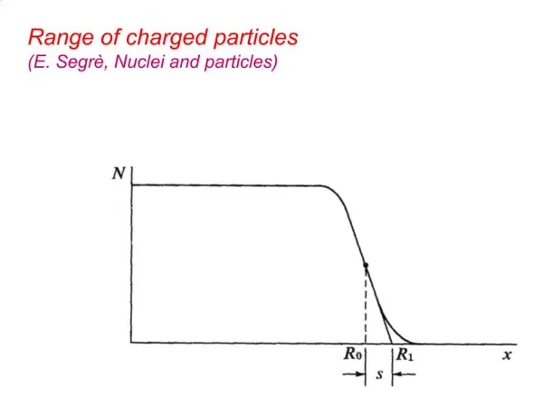
Methods of ParticleIdentification • Lifetime & decay kinematics, eg bottom, charm, etc • Time of flight c (essentially non relativistic) • Energy measurement by calorimetry (essentially non relativistic) • Energy measurement by range (essentially non relativistic) • Cherenkov Radiation. Threshold or angle measurement c • Non relativistic energy loss, dE/dx 1/2 • Relativistic energy loss in gas, dE/dx log() until limited by Density Effect • Transition Radiation for >103 until limited by Formation Zone Effect • Many of these depend on the details of the electromagnetic field of the moving charge which we shall investigate. • Although there are several apparently distinct phenomena, there is only one electromagnetic field. • Therefore there are relationships between the phenomena which are interesting, informative and indeed surprising. Classical EM of Particle Detection
The phenomenology of dE/dx • The rate of energy loss with distance = energy deposited by the charge per metre • dE/dx = 1/velocity * rate of energy loss per unit time • Not a real derivative since actual energy loss collisions subject to statistical fluctuations • 1/2 at low in all materials, • log in low density materials, the “Relativistic Rise”, • the saturation at high log , the Fermi Plateau, the Density Effect 2 1 Relative energy loss 0 1 2 3 log Classical EM of Particle Detection
q c 2 1 Transition Radiation (TR) • A relativistic charge q passes from one dielectric medium to another. • We shall show that the following picturesof TR are in fact equivalent: • The EM field in medium 1 and the EM field in medium 2 do not satisfy the EM boundary conditionsat the surface. To do this a free wave is emitted from the interface. This is TR. • The Cherenkov Radiation (CR) emitted in medium 1 and/or medium 2 is diffracted at the surface ie the CR emission stops/starts there, causing diffraction in the same way as always occurs when a wave is cut off, eg when passing through a slit. This diffracted radiation is TR. • An observer at a distance, either in medium 1 or in medium 2, viewing q passing through the interface would observe an abrupt change in its apparent angular velocity. Such an apparent angular acceleration is always associated with the emission (or absorption) of free radiation. This is TR. Classical EM of Particle Detection
2. Maxwell and Dispersive media2.1 Field of a moving charge in vacuum(traditional) Maxwell’s Equations for a general charge density and current density J: In vacuum due to charge q moving with velocity c and passing through the origin r = 0 at time t = 0, we have Eq 2.1 Eq 2.2 Eq 2.3Eq 2.4 These may not look like wave equations! However the physics is all here. To make the wave equations more explicit, and thence to solve them, let us do some maths (NB there is no physics in the next steps) The maths involves introducing the potentials (A, ). Classical EM of Particle Detection
Eq 2.5Eq 2.6Eq 2.7Eq 2.8 Eq 2.9 Step 1: Maxwell Equations as inhomogeneous wave equations for the potentials (A, ) Equation 2.5 is a (non unique) definition of A whichis equivalent to eq 2.3. Equation 2.6 comes from integrating eq 2.1; theintegration ‘constant’ is any field whose curl is zero. The choice - grad is effectively a definition of . The definition of A can be made unique by choosing its divergence; this choice is called choosing the Gauge. With the Lorentz Gauge the choice is eq 2.9 With this choice eq 2.4 becomes eq 2.7and eq 2.2 becomes eq 2.8. Where has all this messing about got us? Eq 2.5-2.9 are equivalent to Maxwell’s Equations Eq 2.7 & 2.8 are wave equations in and Adriven by the charge and current densities respectively. Eq 2.5 & 2.6 tell us how to get the physical fields from the solutions for and A. How can we solve 2.7 & 2.8? Classical EM of Particle Detection
unit vectors V1 R dV1 Field point, P r1 r O Step 2: Retarded (and Advanced) Potential solutions Equation 2.7 and each component of eq 2.8. They are the same. Consider eq 2.8 as an example. Potential at P due to charge in V1 near origin O. Except in region near O, we have = 0, so The general spherically symmetric solutions of this wave equation due to each dV1 must be of the form The three components of A each have similar solutions. The first term describes outgoing waves emitted by the charges near the origin and is called the Retarded Potential. The second term describes incoming waves absorbed by the charges near the originand is called the Advanced Potential.. Classical EM of Particle Detection
Step 3: The Lienard Wiechert Potentials due to a point charge • We consider just the Retarded Potential f, the emission problem. [The Advanced Potential g, the absorption problem can be found in the same way.] • In the static approximation we have the simple Coulomb potential: • We generalise this to be of the required form ie a function of (R-ct):This shows explicitly that the potential at time t depends on the charge density evaluated, not at time t, but at the earlier time t-R/c, ie at such time that the influence would be reaching the field point r at time t. • Since R varies over V1, the effect is non trivial, even for a point charge, as we now see. • Thus becomes • To get , the density must be integrated over V1 using the identity where and s is the unit vector towards the charge. • The result is the Lienard Wiechert Potentials of a point charge q in terms of variables are evaluated at the earlier “retarded” time, t’ = t - R/c. Classical EM of Particle Detection
2.2 The Feynman Heaviside picture Step 4: The E, B fields In principle the fields are then simply obtained using eq 2.5 & 2.6. However the problem is that the potentials depend on t’, not t. Awkward! The factor dt/dt’ represents a Doppler factor. The method is only applicable in vacuum anyway. Consider first the simpler nonrelativistic case with: The ratio c/R (or rather its transverse part)is the angular velocity of the charge, ds/dt, where (as before) s is the unit vector from the field point or observer to the charge. According to eq 2.5 the transverse electric field at large R is therefore determined by the angular acceleration: Classical EM of Particle Detection
In the relativistic case all we have to do is recall that it is the direction in which the charge appears to be at observer time t that matters. If s’ is the unit vector to the apparent position then at large R: In Volume 1 of his lectures Feynman writes: This is the Feynman-Heaviside formulation of Classical Electrodynamics.The first term is the Coulomb field, the second is the near field or induction field term,the third is the radiation field discussed here which depends only on s’ and not on R.We only need to know the apparent direction of the charge as seen! As Feynman says “That is all - all we need” Classical EM of Particle Detection
The radiation field emitted by a relativistic charge as usually written, for instance in Jackson, looks considerably more complicated! The difference is the relation between real and apparent velocity, and thence between real and apparent acceleration. The relation between real and apparent velocity is the Doppler shift: ThusExtending this argument to the apparent acceleration recovering the messy dependence apparent in standard texts. Conceptually elegant, perhaps, but the Feynman-Heaviside formulation is not very easy to work with. It is important here because we shall need to extend it to radiation problems with media. Classical EM of Particle Detection
2.3 Field of a moving charge in a medium In a medium we need Maxwell’s Equations in their general formfor a general charge density and current density J: These 8 differential equations describe 4 vector fields. The vector fields E and B are distinguished because they can be measured. The force F on a charge q with velocity v is: The vector fields D and H are related; they take account of the dielectric polarisation P and magnetisation M of the medium. In a linear medium this is usually described through the relations: The relative dielectric permittivity and magnetic permeability are unity for vacuum. This suggests that to analyse radiating charges in media all we have to do is substitute 0 for 0 and0 for 0 in the vacuum analysis. However this will not work! The problem is that and are not constants but are functions of frequency. In particular the above relations between D and E (or B and H) are only a deceptive shorthand. Classical EM of Particle Detection
Non local relations between fields Since and are dependent on frequency, they can only be used when is well defined. We shall therefore take the Fourier Transform of the fields thus: Now we say In time this implies the D-E relation: This says that medium takes time to respond to an electric field. The polarisation P (and therefore the D field)at time t depends on the electric field at other (earlier) times.In other words the relation between P & E (also D & E) is not local in time. In fact in a non-uniform medium the relationship is not local in space either. At an atomic level the polarisation depends on the electric field at other places. As a result we have to take the 4-D FT of Maxwell’s Equations themselves to express them in (k, ) space. This may sound awful but actually brings great simplifications! Classical EM of Particle Detection
Each field quantity or its component is related to its 4-D FT labelled with a tilde thus: Examination shows that just brings down a factor ik. In fact all the differential operators become simple factors in (k,) space. Fourier Transformation of field equations The (r,t) equations on the left are transformed into the (k,) equations on the right. Each field is represented by its FT, (k,). Also we have now been able to substitute 0 and 0 for 0 and 0, where and are functions of (k,). 2.10 2.11 2.122.13 2.14 Classical EM of Particle Detection
Fourier Transformation of field equations (continued) These equations are not differential equations - their solution is easy! They do describe the response of a dispersive medium.We can now write down a simple general procedure for finding the fields in a medium for a specific charge and current density. Let us apply the procedure to the case in point, a point charge q moving at constant velocity through the medium..... Classical EM of Particle Detection
Explicit fields of a point charge moving in a medium Step 1. where the first 3 integrations are easy using the -functions. For the fourth we have used: Step 2. Substituting: Steps 3 & 4. In terms of these Note that everything is known except (k,) and (k,). Note also that every field is constrained by (-k.c). Classical EM of Particle Detection
We have not yet learned too much despite the fact that we have an exact result! We need more understanding. What is happening? What are we doing? This will come from simple ideas which explain. We investigate these next. Then later we can put the rigour back into the treatment and achieve both real appreciation and accuracy. Classical EM of Particle Detection
3. The Density Effect, Cherenkov and Transition Radiation in the transparent medium approximation 3.1 A simple 2-D scalar model Consider a scalar field in 2-D (x,y) - and time. Consider a point source moving at constant velocity v along the x-axis. Consider the case in which the field is static in the frame of the source. A familiar example is the wake of a moving boat. The wake is stationary (co-moving) as seen by an observer on the boat. In this frame = 0 but there are waves with kxand ky non zero. The field may be Fourier analysed in the rest frame of the medium, But there is a constraint. The phase of every Fourier component is constant at the source - that is the phase velocity along x equals the velocity of the source v: This is the same condition that we already found for the EM field components, (-k.c). Now we know that it is the condition that the field of a moving charge is static in its rest frame. Classical EM of Particle Detection
y x ky kx Looking at the field component of frequency ω ..... u, phase velocity of field, frequency ω k θ v = βc, velocity of source along x-axis Classical EM of Particle Detection
The phase velocity of waves (call it u) is given by . So by Pythagoras: There are two cases according to whether the root is real or imaginary. v>u, real root In this case ky is real. In the medium frame a real wave is emitted with angleWell known examples: sonic boom, planing speedboat wake, Cherenkov radiation. v<u, imaginary root In this case ky is pure imaginary. The y-dependence of the field is a real exponential, an evanescent wave , as occurs in total internal reflection.The range where Note the relativistic type variables, but note also that no aspects of Relativity have been introduced! Classical EM of Particle Detection
Application of the 2-D scalar model to the EM case In a vacuum the EM phase velocity u = c.There is no free field emission since v is always less than c. The transverse range y0 = , that is the range increases with the relativistic . This field expansion, known as the “Relativistic Expansion”, is, as we see, not peculiarly relativistic or electromagnetic. It is a general feature for any field. In a medium the EM phase velocity u = c/n where is the refractive index. The “optical region” with n > 1, we have both cases:v > u. Shockwave, free emission of Cherenkov Radiation at cos = 1/’ = 1/n andv < u. Evanescent transverse field below Cherenkov threshold with range that expands rapidly as ’ = n approaches 1 The “X ray region” with n < 1, we only have the evanescent case. Indeed at the highest velocity v c, ’ = n and range is Assuming we get range where p is the plasma frequency of the medium. This is a well known result and is responsible for the limited Relativistic Rise of energy loss and the Density Effect. Classical EM of Particle Detection
It is remarkable that such a crude model is able to describe so many of the important features of the actual field. Spatial Dimensions. The model is in 2-D instead of 3-D.In 3-D the waves would be replaced by Bessel Functions (which are closely related to sin/cos and exp functions away from r = 0). Scalar Model. The model is for a scalar not a vector EM field. As we shall see later there is a longitudinal field polarisation which does not show the interesting dependence which is shown by the scalar model.The more interesting transverse field polarisation does behave in the way described by the simple model. Transparent media. Media are necessarily absorptive.We shall see later that the full treatment shows the range effect of the simple model added in quadrature with absorption, as you might naively guess. Consider the field generated by a simple realisation of this 2D model in Mathematica for successively increasing values of v/u..... Classical EM of Particle Detection
0.2 0.3 0.1 1.05 0.97 0.4 0.5 0.6 0.8 0.7 0.95 0.98 0.99 0.995 0.998 0.9 0.999 1.0 1.2 1.1 2.0 1.5 Classical EM of Particle Detection
3.2 The effective mass of the photon • A photon in a medium travels at a velocity c/n, not c as in vacuum. • A “photon” in a medium is a linear combination of a free photon and an electronic excitation of the medium. It is a quantum of a normal mode of these coupled forms. • A photon in a medium is coherently absorbed and re-emitted in the forward direction with a delay depending on how close the frequency is to resonance. • Such a photon is not mass-less. But its mass is a function of frequency!The description is similar to the “electron” in the Band Theory of Solids which is a linear combination (normal mode) of many interacting electrons. Its mass m* me and may be negative (hole states). • The energy is and the momentum is n/c. So • Recall the Yukawa mechanism: exchange of a boson mass m gives potential of range /mc. • Applying this to the range due to the exchange of renormalised photons... Classical EM of Particle Detection
Range of potential due to photon exchange in a medium which is exactly the same result that we obtained from our 2D scalar model. Consider the Optical Region, n > 1.m* is purely imaginary.What does this mean? And what happens to the Range of the exchange force? An imaginary m* or negative m*2 means that the pc > E, in other words we have a space-like 4-vector. OK, nothing wrong with that. The singularity in q2 lies in the physical region for scattering; the propagator goes to infinity at some scattering angle. This is not allowable in vacuum as it would cause divergences. Here m*() and goes to zero at high , so no divergences. OK! Put graphically a photon may be exchanged between the particle and a PhotoMultiplier Tube many metres away! This occurs at a particular q2, ie angle. This is the Cherenkov Effect. The photon may go in the opposite direction; this is a picture of an accelerator. Classical EM of Particle Detection
P-k, E- P, E k, An alternative way to consider this is to ask “What is the condition for a particle to emit a photon?” The incident mass M which emits the photon satisfies Subtracting gives The last term is negligible either because the radiated photon energy is very small compared with E, or because at the energy of the photon n 1. We have taken k = n/c which is true for a free photon. Take the incident energy E = Mc2 and P = Mc, then which is the phase or Cherenkov condition that we have seen twice before. This is the “recoilless” case where the medium takes up no momentum. If the medium has structure (period a), it can absorb recoil momentum rK = r2/aas in Bragg Scattering (r an integer). Such a lattice vibration is called a phonon. Then the condition is generalised . Cherenkov Radiation is r = 0.Transition Radiation is the case r 0. The TR would be diffracted CR....... Classical EM of Particle Detection
3.3 Diffraction and the link between CR and TR Consider a charge q = ze, velocity c, passing through a slab of medium, thickness L and refractive index n(). The number of CR photons N emitted at angle () according to the standard formula [which will be proved later] A B Per unit solid angle d = 2 d(cos), we haveThe finite thickness of the slab implies that the CR wave front is restricted in width (BC in the diagram). The effective slitwidth BC causes the wave to be diffracted around the Cherenkov angle, as in a student Optics Fraunhofer problem... Classical EM of Particle Detection
Fraunhofer Diffraction of CR B C position 1/n cos The phase between the centre and edge of the slit, . The -function is replaced by .If L is large, BC is wide and the broadening of the Cherenkov peak is small.If L is small, the Cherenkov peak can become very broad. Broad enough that, even when the Cherenkov peak is at an unphysical angle (cos > 1), the radiation spreads into the physical region (cos < 1). “Optical Transition Radiation” = sub-threshold Cherenkov Radiation due to Diffraction in a thin foil.[Although the Nobel Prize was given for Optical TR, it is X-ray TR which is important.] This description is qualitatively correct, but we have not proved it yet - because in fact we have made an important mistake.... Classical EM of Particle Detection
Proof that we have made an error: Consider a large number of thin foils of vacuum in sequence. This is obviously just a mathematically sliced vacuum - no radiation. But the above model suggests that there is. Where did we go wrong?The fields from a physical foil in vacuum should be seen as the effect of substituting a foil of material for a foil of vacuum. So we need to square the difference of amplitudes (as above) for the foil and the medium in which it is immersed (we shall assume that this is vacuum, but that is not necessary).The Principle of Superposition tells us that we should have thought of this before. We need to make another change.CR is typically observed within the medium at angle , see previous diagram.TR is analysed outside the medium at angle , so that refraction (Snell’s Law) has accounted for: With these changes Classical EM of Particle Detection
Note 1. In the big round bracket the first term has a pole at condition for CR in foil. This term is the Optical TR effect already discussed. Note 2. In the big round bracket the second term has a pole at condition for CR in vacuum (in general, the surrounding medium). The singularity is truly at = 1, exactly what we need for particle identification. It is responsible for X-ray TR and its linear dependence on . Note 3. The sin2[] term with argument represents the interference between two waves amplitude A and -A emitted at the front and back surfaces of the foil with phase difference 2. The fluxfrom one interface in the absence of interference (A2) would be Classical EM of Particle Detection
Note 4. To discuss X-ray TR from a foil we make some approximations. Then the number of photons emitted from the foil is This is a very important result because it is the very formula to be found in the literature for Xray TR from a foil. From the way in which we derived it we may conclude that Transition Radiation ISFraunhofer Diffracted Cherenkov Radiation.It is a useful and practical formula, although it ignores the effects of absorption and scattering.The flux is small (see next slide) at angles greater than a few times 1/, justifying the small angle approximation already made.As before the flux from one interface is obtained by dropping the 4sin2 factor. Classical EM of Particle Detection
Angular distribution of Xray TR from a single interface In the small angle approx d = 2 d. The angular distribution of energy S is dSd 100 1 0.01 =25000 =5000 =1000 0.01 0.1 1 10 mradians Classical EM of Particle Detection
12 dS 103dE 8 4 0.2 0.4 0.6 0.8 a=E/Ep The spectrum of Xray TR from an interface This is seen to be a universal function of the scaled spectral energy variable a. Most of the flux is emitted with energy less than 0.5Ep. Recall that where N is the electron density.If the flux is to escape the foil, this energy must be much greater than the K-edge. Classical EM of Particle Detection
The integrated flux of Xray TR from an interface Integrating the found angular distribution of energy , yields a total flux The typical TR photon has energy of order Ep/4. (as shown previously by the spectrum). The number of TR photons per interface is of order z2 So the hardness of the TR photons increases linearly with and the root of the electron density. These conclusions have to be modified by a) absorption [our model is transparent!]b) the interference factor which can be written 4sin2(L/Z) where the Formation Zone, Z, is given by If L < Z, the TR is said to be in the first Formation Zone (cf the principal max in Fraunhofer Diffraction). If L « Z, the TR is killed by the destructive interference. Since ~1/, p/~1/, roughly . This implies a minimum L which increases quadratically with . Problem What is the smallest value of for which you would expect TR to be observable from radiators of a)lithium b)carbon? How thick must they be? Classical EM of Particle Detection
Conclusion on the relationship between CR and TR We have derived a correct description of TR by integrating the CR radiation along a finite length of track. This tells us that TR is an integral representation of the EM field, whereas CR is a differential representation. They are related as indefinite integral (to be evaluated and subtracted at the two ends of the track) to integrand (to be summed along the track length). They are different ways of describing one phenomenon. Classical EM of Particle Detection
3.4 CR and TR as radiation from an apparently accelerating charge Remember that in vacuum we found the Feynman Heaviside formulation for the radiation seen by P observing charge q:1. Calculate s’(t), the unit vector in the apparent direction of q as seen by P at time t2. Calculate its second time derivative with respect to observer time t.3. The observed radiated E and B fields are then 4. Fourier analyse E and B in time5. Calculate the energy flux seen by P as a function of 6. Calculate the photon flux by dividing by Problem An observer P sees a charge q = Ze undergo a discontinuity in its apparent transverse angular velocity ds’/dt. Show that the observer P sees a photon flux Now, provided that the observer P is in free space, the same method can be applied when there are media. All we need are the apparent movements of the apparent charges. This gives us a new and revealing picture of CR and TR. Classical EM of Particle Detection
The observer looks at CR Moving source Q as seen by the observer at P.Until the Cherenkov cone reaches him P sees nothing. Classical EM of Particle Detection
After the cone passes him P sees two charges, one at F1 and one at B1 Classical EM of Particle Detection
Later P sees the charges at F2 and B2. Evidently F1 and F2 appears as a forward-going charge, while B1 and B2 describe a backward-going one Classical EM of Particle Detection
Time since charge was at closest approach F = t, so FE = ctCE = CF + FE = b cot + ctBut CE is how far the source went in the time that the light covered CB (= b cosec )ThusCE = n CBSubstituting gives the implicit dependence of on t that we need to get d2/dt2: The formula for the flux of Cherenkov Radiation can be derived from this. However the maths involves a difficult integration which we will not follow here. So what the observer sees is nothing and then two charges moving away from one another. Since charge is locally conserved, it appears conserved on any space-time surface - the backward-going charge is -Q and the forward-going charge is +Q. The observer sees the creation of a charge dipole and therefore detects the corresponding radiation. The physical picture is clear. We need the apparent angular charge acceleration. The distance of closest approach BF = b Classical EM of Particle Detection
Therefore at a distance r a discontinuity in apparent transverse angular velocity ds’/dt is seen,and hence radiation The observer looks at TR When in vacuum the observer sees the charge moving with an apparent transverse velocity When in the medium, index n, the apparent transverse velocity (geom + Snell’s Law) Classical EM of Particle Detection
If we make the Xray TR approximations we had before, namely this becomes This is the result for the TR from a single interface that we deduced before by considering the effect of diffraction on CR. We may conclude that TR can be visualised and calculated as due to the apparent acceleration of charge at an interface. In fact we can calculate the flux without approximations, but we need a bit more care.... Classical EM of Particle Detection
Exact calculations of TR at a single interface Before the charge crosses the surface,apparent charge q1 with apparent transverse vel v1 After the charge crosses the surface,apparent charges q2 and q3 with apparent transverse vel v2 and v3 v1 and v2 are as before and v3 = - v2 If f=q3/q2and q2=ze, then q1 =(1+f) q2 (charge conservation); Classical EM of Particle Detection
4. Energy Loss in Absorptive Media 4.1 Phenomenology of Electromagnetic Media In the foregoing we have said almost nothing about the medium, simply characterising it by the refractive index, n. The dependence of n on and the relation between the real and imaginary parts are crucial - after all detector signals arise from the absorption of electromagnetic energy. Constituent and Resonant Scattering EM waves interact with a) medium constituents and b) composite structures. The former is called Constituent Scattering, has a typically small and energy independent cross section.The latter is called Resonance Scattering, has a large and energy dependent cross section.At the energies of interest here the constituents are electrons and nuclei, the composites are atoms and molecules. Classical EM of Particle Detection