Download
1 / 35
430 likes | 653 Views
Numerical Models. Outline Types of models Discussion of three numerical models (1D, 2D, 3D LES). Types of River Models (1). Conceptual Qualitative descriptions and predictions of landform and landscape evolution e.g., “cartoons” and +/- relationships Empirical

E N D
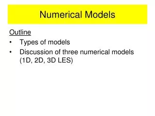
Numerical Models Outline • Types of models • Discussion of three numerical models (1D, 2D, 3D LES)
Types of River Models (1) • Conceptual • Qualitative descriptions and predictions of landform and landscape evolution • e.g., “cartoons” and +/- relationships • Empirical • Functional relationships based on data • May include statistical relationships • e.g., hydraulic geometry • Analytical • Derive new functional relationship based on physical processes and conservation principles (mass, energy, momentum); deterministic • e.g., sediment transport equations
Types of River Models (2) • Numerical • Represents all relevant physical processes in a set of governing equations • Conservation of fluid mass, energy, momentum (fluid and sediment) • 1D, 2D, or 3D; dynamic; coupled or decoupled, science of numerical recipes • Cellular Automata • Cells of a lattice that interact according to rules based on abstractions of physics
Discussion of Three Models • 1D numerical model routes flow and sediment along a single channel • 2D numerical model that routes flow and sediment within curved channels • 3D Large Eddy Simulation (LES) model that routes flow in complex channels
1D Numerical Model • Route flow and sediment (decoupled) in a straight, non-bifurcating alluvial channel • 1D: width- and depth-averaged • Primary purpose: To address erosion, transport, and deposition of sediment (sorting processes and bed adjustment) • MIDAS: Model Investigating Density And Size sorting
MIDAS (van Niekerk et al., 1992a,b) Q-flow discharge; S0-bed slope, Sf-friction slope, R-hydraulic radius, ks-roughness height, w-settling velocity, ijk-coefficients for gain size and density, and bed shear stress, F-proportion of ij, P-proportion of shear stress k
MIDAS (van Niekerk et al., 1992a,b) • Treatment of bed: • Active layer: what is available for transport in a given time- and space-step • Particle exchange between active layer and moving bed occurs during each time-step; grain size-density distributions are adjusted • If degradation occurs: active layer is replenished from below • If deposition occurs: active layer moves upward • Assume fluid flow and sediment transport are over time-step
MIDAS (van Niekerk et al., 1992a,b) Numerical Procedure (at every x, then t): Gradually varied flow equation solved using standard step-method, subject to downstream boundary condition and n Shear stress (and bedload transport (ib) determined From ib, determine suspended load Bed continuity equation solved at each node using a modified Preissmann scheme (nearly a central [finite] difference scheme) New grain size-density distributions, as modified by erosion or deposition
Degradation (Bennett and Bridge, 1995) Equilibrium Equilibrium; steady, uniform flow Post- degradation Post- degradation; steady, nonuniform flow
(Bennett and Bridge, 1995) Aggradation Eq. Post- Agg.
2D Numerical Model • Route flow and sediment (decoupled) in a straight to mildly sinuous, non-bifurcating alluvial channel with vegetation • 2D: depth-averaged • Depth-integrating the time- and space averaged 3D Navier-Stokes equations • Considers the dispersion terms associated with helical flow • Explicitly addresses the effects of vegetation in stream corridor
Depth-averaged 2D numerical model (Wu et al., 2005)
Depth-averaged 2D numerical model (Wu et al., 2005)
Depth-averaged 2D numerical model (Wu et al., 2005) Numerical Procedure: Governing equations are discretized using a finite volume method on a curvilinear, non-orthogonal grid for flow and sediment Bed is discretized using finite difference in time at cell centers Flow and sediment are decoupled • Two applications: • Little Topashaw Creek, MS; channel adjustment to LWD structures • Physical model of alluvial adjustment to in-stream vegetation
LWD (a) Map of study site, Little Topashaw Creek; (b) Photo facing upstream. Shaded polygons are large wood structures Little Topashaw Creek, MS (Wu et al., 2005)
Little Topashaw Creek, MS Computational Grid Computational grid used in simulating LTC bend. (Wu et al., 2005)
Little Topashaw Creek, MS Flow Vectors Simulated flow field at LTC bend (Q=42.6 m3/s) (Wu et al., 2005)
Simulated Flow, Little Topashaw Creek, MS Without LWD With LWD (Wu et al., 2006)
Measured and simulated bed changes between June 2000 and August 2001. Units of bed change and scale are m, and the contour interval is 0.25 m. Little Topashaw Creek, MS Bed Adjustment deposition erosion (Wu et al., 2005)
Physical Model (Bennett et al., accepted)
Physical Model (Bennett et al., accepted)
Physical Model Bed Adjustment Observed Predicted Contour plots of changes in bed surface topography in response to the rectangular vegetation zone with VD = 2.94 m-1 as (a) observed in the experiment and as (b) predicted using the numerical model. Flow is left to right. (Bennett et al., accepted)
Physical Model Flow Vectors Predicted Simulated depth-averaged flow vectors for the trapezoidal channel with (a) no vegetation present, and in response to the rectangular vegetation zone (shown here as a lined box) at a density of 2.94 m-1 at (b) the beginning and (c) conclusion of the experiment. (Bennett et al., accepted)
Physical Model Bed Shear Stress Predicted Contour plots of simulated distributions of bed shear stress for the trapezoidal channel with (a) no vegetation present, and in response to the rectangular vegetation zone (shown here as a lined box) at a density of 2.94 m-1 at (b) the beginning and (c) conclusion of the experiment. Flow is left to right. (Bennett et al., accepted)
3D Numerical Models • Classic in 3D modeling is to close the Navier–Stokes equations by: • Reynolds decomposition of the velocity components into mean and fluctuating components • Employ a Boussinesq approximation to link the resulting Reynolds stresses to properties of the time-averaged flow (Reynolds-averaged Navier–Stokes (RANS) approach) • Mixing-length model is one such closure scheme where the characteristic length and timescales of the turbulence are prescribed a priori • So-called k–e model still the most popular way of determining these length and timescales from properties of the flow • RANS focused on the accurate representation of the mean flow field
3D Numerical Models • Large Eddy Simulation (LES) resolves the turbulence above a particular filter scale, rather than resolving variations greater than the integral timescale as occurs in RANS • Can yield accurate results in situations where turbulent structures of importance to the modeler are generated at a variety of scales • LES calculates the properties of all eddies larger than the filter size and models those smaller than this scale by a subgrid-scale (SGS) turbulence transport model
3D LES Model • LES equations are derived by applying a filter to the Navier–Stokes equations • RANS approaches to modeling the Navier–Stokes equations decompose the velocity in to mean and fluctuating components, whereas LES is based upon a length scale for a filter, often taken to be equal to the grid size employed • Important differences of LES vs. RANS • LES equations retain a time derivative (why LES can be employed to give time-transient solutions) • Additional stress term contains more components than the Reynolds stresses in RANS (Smagorinsky SGS model is most commonly used for subgrid-scale solutions)
Flow past Groynes (McCoy et al 2007) Mean velocity streamlines visualizing vortices inside the embayment region
Flow past Groynes (McCoy et al 2007) Mean velocity streamlines visualizing vortex system in the downstream recirculation region
Flow past Groynes Instantaneous contours of contaminant concentration at groyne middepth (upper) and midwidth (lower) (McCoy et al 2007)
Flow past Plant Stem (cylinder) Visualization of horseshoe vortex system in the mean flow and associated upwelling motions downstream of the plant stem a) flat bed b) deformed bed Visualization of the tornado-like vortex inside the recirculation region on the right side of the plant stem using 3-D streamlines (flat bed case). (Neary et al., submitted)
Turbulent Flow over Fixed Dunes (Bennett and Best, 1995)
Flow over Dune: LES Instantaneous velocity fluctuation fields of u and w in the middle plane of the channel. Dashed lines represent the instantaneous free-surface positions. Q2 and Q4 stand for quadrant two and four events Three-dimensional view of instantaneous flow, where shadow area represents free surface, view of upper-half channel, and magnified view of free surface, where the labels U and D represent upwelling and downdraft. (Yue et al., 2005a) (Yue et al., 2005b)
Fluvial Models and River Restoration • Future of stream restoration relies heavily upon advancing current modeling capabilities (tools) • Use models to verify field and laboratory data • Use models to assess various restoration strategies (rapidly, cheaply, and without harm to the environment)
Fluvial Models • Conclusions • 1D models provide readily available quantitative information of erosion, transport and deposition within river corridors in the downstream direction, but not laterally • 2D and 3D models provide the highest fidelity of turbulent flow in downstream and lateral directions (as well as vertical directions with 3D codes), but require • Much expertise in fluid mechanics and numerical techniques • Much computer capability