Download
1 / 52
520 likes | 720 Views
Short Run. Decision Time Frames. The actions that a firm can take to influence the relationship between output and cost depend on the time frame. Short run: The quantity of at least one input, (ie: factory size) is fixed and the quantities of the other inputs, (ie: Labour) can be varied.

E N D
Short Run Decision Time Frames • The actions that a firm can take to influence the relationship between output and cost depend on the time frame. • Short run: The quantity of at least one input, (ie: factory size) is fixed and the quantities of the other inputs, (ie: Labour) can be varied. (short run decisions are easily reversed: there is no time to go in and out of business)
Long Run • Long run: the quantities of all inputs can be varied, nothing is fixed, (ie: plant size can vary.) (long-run decisions are not easily reversed: new firms can enter and old firms can leave; that is, firms can go in and out of business) Decision Time Frames • Firms make two kinds of decisions: • Short Run decisions govern the day to day operations of the firm • Long Run decisions involve longer term strategic planning
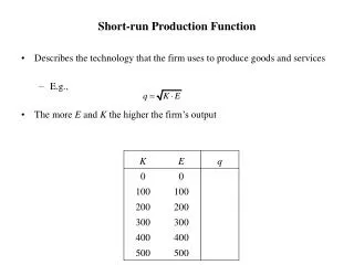
The Costs of Production: Short Run • S.R. Production Function • the relationship between quantity of inputs used to make a good and the quantity of output when some factors are fixed and some are variable
Total, Marginal, & Average Product MP=DTP/DQL AP=TP/QL
Total Product & Marginal Product TP d 13 c 10 MP 2 3 • as TP , & MP ¯, TP increases at a decreasing rate 15 6 13 • total product (TP) always increasing 10 4 Marginal product (sweaters per day per worker) 3 3 Output (sweaters per day) 5 2 4 0 1 2 3 4 5 0 1 2 3 4 5 2 3 Labour (workers per day) Labour (workers per day)
Marginal Product • Law of diminishing returns • As a firm uses more of a variable input, with a givenquantity of fixedinputs, themarginal productof thevariable inputeventuallydiminishes. Similar to diminishing Marginal Utility for consumers.
The Relationship Between a Firm’s Output and Costs in the Short Run Per Unit Costs To produce more output in the short run, the firm must employ more variable factor, for example, labour, which increases its costs. There are three types of costs: Total Costs Marginal Cost Average Cost
1.)Total Costs: TC = TFC + TVC Total Total fixed variable Total cost cost cost Labour Output (workers (sweaters (TFC) (TVC) (TC) per day) per day) (dollars per day) a 0 0 b 1 4 c 2 10 d 3 13 e 4 15 f 5 16 25 25 25 25 25 25 0 25 50 75 100 125 25 50 75 100 125 150
Total Costs TC TC = TFC + TVC 150 TVC Cost (dollars per day) 100 50 TFC 0 5 10 15 Output (sweaters per day)
2.)Marginal Cost Total Total fixed variable Total cost cost cost Labour Output (workers (sweaters (TFC) (TVC) (TC) per day) per day) (dollars per day) Marginal cost (MC) 0 25 50 75 100 125 25 25 25 25 25 25 a 0 0 b 1 4 c 2 10 d 3 13 e 4 15 f 5 16 25 50 75 100 125 150 6.25 4.17 8.33 12.50 25.00 the in total cost that results from a one-unit in output. MC = TC TO MC = TVC Q
Avg. fixed cost (AFC) TFC/Q Avg. variable cost (AVC) TVC/Q Avg. total cost (ATC) TC/Q — 6.25 2.50 1.92 1.67 1.56 — 6.25 5.00 5.77 6.77 7.81 — 12.50 7.50 7.69 8.33 9.38 3.)Average Cost Total Total fixed variable Total cost cost cost Labour Output (workers (sweaters(TFC) (TVC) (TC) per day) per day) Marginal cost (MC) (dollars per day) a 0 0 b 1 4 c 2 10 d 3 13 e 4 15 f 5 16 25 25 25 25 25 25 0 25 50 75 100 125 25 50 75 100 125 150 6.25 4.17 8.33 12.50 25.00
Marginal Cost and Average Costs MC ATC AVC AFC 25 ATC = AFC + AVC 15 10 Cost (dollars per sweater) 5 0 5 10 15 Output (sweaters per day)
Marginal Cost and Average Costs MC 25 MC ¯ at low outputs due to gains from specialization, MC eventually due to law of diminishing returns. 15 10 Cost (dollars per sweater) 5 0 5 10 15 Output (sweaters per day)
Relationship between MC & ATC Whenever MC < ATC, ATC MC > ATC, ATC • MC crosses ATC at the minimumATC (capacity or minimum efficient scale) • MC crosses AVC at the min. point
Shifts in the Cost Curves The position of a firm’s short-run cost curves depends on two factors: • technology • prices of resources
Long Run Costs of Production • In the long run, all factors ofproduction are variable, • nothing is fixed. • In the long run, firms are looking forproductive efficiency, • producing a given quantity at as low a • per unit cost as possible. • assuming a constant state of technology • and constant resource/input prices.
The long run is the firm’s planning perspective while the short run is the firm’s operating perspective.
The Long-Run Average Cost Curve • The long-run average cost curve shows the relationship between the lowest attainable average total cost and output • It is therefore derived from the short-run average total cost curves. • Each SRATC touches the LRATCat the level of output for which the quantity of the fixed factor is optimal and lies above the LRATC for all other levels of output.
Preferable Plant Size and theLong-Run Average Cost Curve SAC4 SAC5 SAC3 SAC6 SAC2 SAC1 SAC7 SAC8 SAC1 SAC2 C2 Average Cost (dollars per unit of output) LAC envelope C4 C1 C3 SAC3 Q1 Q2 Build plant 1 if expected output at Q1. Average Cost (dollars per unit of output) Build plant 2 if expected output at Q2. Output per Time Period Output per Time Period
Long-Run Average Cost Curve ATC2 ATC1 ATC3 ATC4 Least-cost plant is 1 LRACcurve Least-cost plant is 2 Least-cost plant is 3 Least-cost plant is 4 18 24 • Once the plant size is chosen, the firm operates on the short-run cost curves that apply to that plant size. 12.00 10.00 8.00 6.00 0 5 10 15 20 25 30
Shape of LRAC & Returns to Scale • Returns to scale are the increases in output that result from increasing all inputs by the same percentage. • There are 3 Possibilities. 1)Increasing Returns to Scale or Economies of Scale: 2)Decreasing Returns to Scale or Diseconomies of Scale: 3)Constant Returns to Scale
Long-Run Average Cost Curve Diseconomies of scale Economies of scale MES LRAC curve Minimum efficient scale: the smallest quantity of output at which LRATC reaches its lowest level. 12.00 10.00 8.00 6.00 18 24 0 5 10 15 20 25 30
What would cause LRATC to shift? 1) change in the state of technology 2) change in input prices Question • What is the difference between diminishing returns (MP) and diminishing returns to scale?
Perfect Competition • A market structure in which the decisions of individual buyers and sellers have no effect on market price No one person in the market has any Market Power: the ability to influence the price. • the minimum efficient scale is small relative to the demand for a good or service.
Characteristics of a Perfectly Competitive Market Structure 1.)Large number of buyers and sellers • no one buyer or seller has power to influence price • Both firms and buyers are “price takers” 2) Homogenous products • goods offered by various producers are largely the same. 3) No barriers to entry or exit 4) Buyers and sellers have equal information
Demand, Price, and Revenue in Perfect Competition FIRM 50 Sidney’s demand curve 25 MR Price (dollars per sweater) 0 9 20 Quantity (sweaters per day) Sidney’s demand and marginal revenue INDUSTRY S 50 Market demand curve Price (dollars per sweater) 25 D 0 9 20 Quantity (thousands of sweaters per day) Sweater market
Demand, Price, and Revenue in Perfect Competition: Firm Total revenue (TR = PxQ) (dollars) Quantity sold (Q)(sweaters per day) Price (P) (dollars per sweater) Marginal revenue (MR =DTR/DQ) (dollars) 25 25 200 225 250 8 9 10 25 25 25
Economic Profit and Revenue: Firm Marginal revenue (MR) is the change in revenue resulting from a one-unit increase in output sold. • For the firm, in perfect competition, • since the price remains constant when the quantity sold changes • Marginal revenue equals price. • marginal revenue curve is also the demand curve. • Demand is perfectly elastic.
Demand, Price, and Revenue in Perfect Competition 50 Sidney’s demand curve 25 MR=P Price (dollars per sweater) 0 9 20 Quantity (sweaters per day) Sidney’s demand and marginal revenue Market Price = $25 INDUSTRY FIRM S 50 Market demand curve Price (dollars per sweater) 25 D 0 9 20 Quantity (thousands of sweaters per day) Sweater market
Firm Maximizes Profits: “Supply” A firm will produce the level of output that maximizes economic profits given the constraints it faces. • market constraints summarized by its revenue schedules. • technology & cost constraints summarized by its product & cost curves.
Profit Maximization Rule MR MC • Produce all those units of output that add more to revenues than to costs. • Produce more output until MR comes closest to being equal to MC without MC exceeding MR:
FIRM Total Revenue, Total Cost, & Economic Profit Total Cost (TC) (dollars) Economic Profit (TR - TC) (dollars) Average Total Cost (ATC) (dollars) Average Var. Cost (AVC) (dollars) Marginal Cost (MC) (dollars) Marginal Revenue (MR) (dollars) Total Revenue (TR) (dollars) Quantity (Q) (sweaters /day) 0 45.00 33.00 28.33 25.00 22.80 21.00 20.14 20.00 20.33 21.00 22.27 25 27.69 0 23.00 22.00 31.50 19.5018.40 17.33 17.00 17.25 17.89 18.89 20.27 23.17 26.00 0 23.00 21.00 19.00 15.00 14.00 12.00 15.00 19.00 23.00 27.00 35.00 55.00 60.00 0 25.00 25.00 25.00 25.00 25.00 25.00 25.00 25.00 25.00 25.00 25.00 25.00 25.00 0 1 2 3 4 5 6 7 8 9 10 11 12 13 22 45 66 85 100 114 126 141 160 183 210 245 300 360 0 25 50 75 100 125 150 175 200 225 250 275 300 325 -22 -20 -16 -10 0 11 24 34 40 42 40 30 0 -35 P=MR
Between zero output and MC = MR output, MR > MC, TR is increasing more than TC, and profits are increasing. Profit-Maximizing Output Profit- maximization Point, MC=MR MR MR > MC MC > MR FIRM Market Price = $25 MC 30 25 $’s.Marginal revenue and marginal cost • Beyond MC=MR output, MC>MR, TC is increasing more than TR, and profits are decreasing. 20 10 0 8 9 10 Quantity (sweaters per day)
FIRM Economic Profit ATC Economic profit Note: In Perfect Competition, MR=AR Market Price = $25 30.00 MC 25.00 MR At P = $25, ATC =$ 20.33 Output = 9 units TR = $25 x 9 = $225 TC = $20.33 x 9 =$183 Profit = $225-$183=$42 Profit = (P-ATC) x output Price and cost (dollars per sweater) 20.33 15.00 0 9 10 Quantity (sweaters per day)
Demand, Price, and Revenue in Perfect Competition MR Market Price = $20 FIRM INDUSTRY Sidney’s new demand curve Sidney’s demand curve 50 S 50 New market demand curve Price (dollars per sweater) Price (dollars per sweater) 25 25 MR 20 20 D D 0 9 20 0 9 20 Quantity (sweaters per day) Quantity (thousands of sweaters per day) Sidney’s demand and marginal revenue: firm Sweater market: Industry
FIRM Total Revenue, Total Cost, and Economic Profit New Price Total Cost (TC) (dollars) Economic Profit (TR - TC) (dollars) Average Total Cost (ATC) (dollars) Average Var. Cost (AVC) (dollars) Marginal Cost (MC) (dollars) Marginal Revenue (MR) (dollars) Total Revenue (TR) (dollars) Quantity (Q) (sweaters /day) -22 -25 -26 -25 -20 -14 -6 -1 0 -3 -10 -25 -60 -100 0 45.00 33.00 28.33 25.00 22.80 21.00 20.14 20.00 20.33 21.00 22.27 25 27.69 0 23.00 22.00 31.50 19.5018.40 17.33 17.00 17.25 17.89 18.89 20.27 23.17 26.00 0 23.00 21.00 19.00 15.00 14.00 12.00 15.00 19.00 23.00 27.00 35.00 55.00 60.00 0 20.00 20.00 20.00 20.00 20.00 20.00 20.00 20.00 20.00 20.00 20.00 20.00 20.00 0 1 2 3 4 5 6 7 8 9 10 11 12 13 22 45 66 85 100 114 126 141 160 183 210 245 300 360 0 20 40 60 80 100 120 140 160 180 200 220 240 260
Break-Even Price P=$20; ATC=$20 TR = $20X8 units/day = $160 TC = $20X8units/day = $160 TR = TC = 0 Economic Profits FIRM Short-Run Break-Even Price ATC Break-even Point, MR=MC=ATC 20.00 MR Market Price = $20 30.00 MC 25.00 Price and cost (dollars per sweater) 15.00 0 8 10 Quantity (sweaters per day)
FIRM Short-Run Losses, & Shutdown Price • What do you think? • Would you continue to produce if you were incurring a loss? • What if price fell to $19.00? • What if price fell to $16.00 or lower?
Demand, Price & Revenue: Perfect Competition MR1 Market Price = $19 INDUSTRY FIRM Sidney’s new demand curve 50 S 50 New market demand curve Price (dollars per sweater) Price (dollars per sweater) 25 25 MR2 20 20 MR3 19 19 D1 D3 D2 0 9 20 0 9 20 Quantity (sweaters per day) Quantity (thousands of sweaters per day) Sidney’s demand and marginal revenue: Firm Sweater market: Industry
FIRM Total Revenue, Total Cost, and Economic Profit 0 45.00 33.00 28.33 25.00 22.80 21.00 20.14 20.00 20.33 21.00 22.27 25 27.69 0 23.00 22.00 31.50 19.5018.40 17.33 17.00 17.25 17.89 18.89 20.27 23.17 26.00 0 23.00 21.00 19.00 15.00 14.00 12.00 15.00 19.00 23.00 27.00 35.00 55.00 60.00 0 19.00 19.00 19.00 19.00 19.00 19.00 19.00 19.00 19.00 19.00 19.00 19.00 19.00 0 1 2 3 4 5 6 7 8 9 10 11 12 13 22 45 66 85 100 114 126 141 160 183 210 245 300 360 0 19 38 57 76 95 114 133 152 171 190 209 228 247 New Price Total Cost (TC) (dollars) Economic Profit (TR - TC) (dollars) Average Total Cost (ATC) (dollars) Average Var. Cost (AVC) (dollars) Marginal Cost (MC) (dollars) Marginal Revenue (MR) (dollars) Total Revenue (TR) (dollars) Quantity (Q) (sweaters /day) -22 -51 -28 -28 -24 -19 -12 -8 -8 -12 -20 -36 -72 -113
FIRM SR Economic Loss Minimization ATC loss Market Price = $19 • Loss Min,P=$19.00 • MC = MR @ 8 units • ATC ($20) > P ($19); Losses = $8 • TFC = $22.00 • Shut down, • lose $22.00 • Produce, lose $8 • Minimize losses by producing when • P >AVC <ATC 30.00 MC 25.00 AVC Price and cost(dollars per sweater) 20.00 19.00 MR 8 10 0 Quantity (sweaters per day)
FIRM Total Revenue, Total Cost, and Economic Profit 0 45.00 33.00 28.33 25.00 22.80 21.00 20.14 20.00 20.33 21.00 22.27 25 27.69 0 23.00 22.00 31.50 19.5018.40 17.33 17.00 17.25 17.89 18.89 20.27 23.17 26.00 0 23.00 21.00 19.00 15.00 14.00 12.00 15.00 19.00 23.00 27.00 35.00 55.00 60.00 0 16.00 16.00 16.00 16.00 16.00 16.00 16.00 16.00 16.00 16.00 16.00 16.00 16.00 0 1 2 3 4 5 6 7 8 9 10 11 12 13 22 45 66 85 100 114 126 141 160 183 210 245 300 360 0 16 32 48 64 80 96 112 128 144 160 176 192 208 New Price Total Cost (TC) (dollars) Average Total Cost (ATC) (dollars) Average Var. Cost (AVC) (dollars) Marginal Cost (MC) (dollars) Marginal Revenue (MR) (dollars) Total Revenue (TR) (dollars) Quantity (Q) (sweaters /day) Economic Profit (TR - TC) (dollars) -22 -29 -34 -37 -36 -34 -30 -29 -32 -39 -50 -69 -108 -152
FIRM Short Run Shut Down loss Market Price = $16 Shutdown:P=$16.00 • MC = MR @ 7 units • ATC (20.14) > P ($16): • Losses = $29.00 • TFC = $22.00 • Shut down, lose $22 • Produce, lose $29 • Minimize losses by shutting down when • P AVC at MC = MR 30.00 MC ATC 25.00 Price and cost(dollars per sweater) AVC 20.14 16.00 MR 0 7 10 Quantity (sweaters per day)
FIRM Short Run Supply • Def’n: Quantity that producers will produce at various possible prices in a set of prices, for a given time period: ceteris paribus. • At each price a firm will produce the output for which MC comes closest to being equal to MR without MC exceeding MR &…….
A Firm’s SR Supply Schedule MC=Supply Profit point MR3 Break-even point MR2 Shutdown point MR1 Minimize losses MR0 MC 31 Price and cost (dollars per sweater) 25 20 17 0 7 8 9 10 Quantity (sweaters per day)
“Supply” FIRM • The Short Run “supply” schedule of the firm is found to be the “MC” schedule • but with 2 qualifications.
FIRM Qualifications 30.00 MC AVC 25.00 Price and cost (dollars per sweater) MR 15.00 0 8 10 Quantity (sweaters per day) • 1.) Only the • upward sloping • part of MC • qualifies • as the SR “supply” • 2.) Only that • part of the MC • that lies above • the AVC • qualifies as the • SR “supply”
Market Supply • Total amount provided to the market at each possible price… • Or • The marginal cost of providing additional output to the market, given current production conditions.
Market Supply • Note: In the SR, quantity supplied is positively related to price for 2 reasons: • As the market price increases, • 1.) each firm uses its capital more intensively thereby increasing output, but also increasing marginal cost. • 2.) firms that were previously providing output but had ceased production, to minimize losses, will find it profitable to begin production again, using capital that had been idle.