Download
1 / 30
330 likes | 440 Views
The formation and dynamics of cold-dome northeast of Taiwan. Mao-Lin Shen, Yu-Heng Tseng and Sen Jan 2014/8/21. Outline. Introduction Numerical model Observation Numerical results Mechanism analysis Conclusion. Introduction (1/3).

E N D
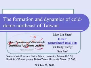
The formation and dynamics of cold-dome northeast of Taiwan Mao-Lin Shen, Yu-Heng Tseng and Sen Jan 2014/8/21
Outline • Introduction • Numerical model • Observation • Numerical results • Mechanism analysis • Conclusion
Introduction (1/3) • An active upwelling area and nutrient-rich (Chen, 1992; Hsu, 2005) • The exchange of Kuroshio Water and Continental Water of East China Sea (Isobe, 2008; Matsuno et al., 2009) • Temperature lower than surrounding about 3~6℃. • Observations have been well-documented by Chern and Wang (1989), Gong et al. (1992), Lin et al. (1992), Tang and Tang (1994), Chen et al. (1995) and Tang et al. (1999), etc.
Introduction (2/3) Fig. 1. Distribution of the centroid of cold patch formed between 2003-2008. Red stars denote the distribution of cold patch in summer (June to October) and green stars show that in winter. (Cheng et al., 2009)
Introduction (3/3) • Water mass properties (Chen et al., 1995): • Kuroshio Surface Water (KSW) dominate surface region in winter. • Kuroshio Tropical Water (KTS) and Kuroshio Intermediate Water (KIW) participate mainly in summer. • Wind disturbance has been considered by Gong et al. (1992), Chang et al. (2009) and Chang et al. (2010). • Using field measures reveal the properties of cold-dome and model output to verify the mechanism of cold-dome formation.
Numerical model (1/3) • Dietrich/Center for Air Sea Technology (DieCAST) hydrostatic ocean model • Surface sources of heat and fresh water • Levitus94 seasonal climatology • Bathymetry • unfiltered ETOPO-2 depth data supplemented with the Taiwan’s NCOR 1-minute high accuracy depth archive in the Asian Seas • Winds stress • monthly Hellerman and Rosenstein winds stress • Vertical mixing • parameterized by eddy diffusivity and viscosity using a modified Richardson number dependent formula based on Pacanowski and Philander (1981)
Numerical model (2/3) ─ Governing Equations • Conservation of mass • Horizontal momentum equations • Equation of conservation of salt or energy (potential temperature) • State equation: • Hydrostatic equation: (1) (2) (3) (4) (5) (6)
Numerical model (3/3) ─ Domain Fig. 2. Schematic of the whole domain under consideration
Take for calculating the Time-longitude plot. Observation (1/5)─ MW and IR mergrd SST 30 July 2008 Typhoon Fung-Wong (28 July) just pass. 16 May 2008 7 November 2009 2 May 2009 Fig. 3. The SST image around the vicinity region. The dark red encircled lines indicate Cold-Dome Favorite Region (CDFR). The fronts identify the boundary of warm water carried by Kuroshio and the cold water remained on continental shelf or the cold-dome.
Observation (2/5)─ Time-longitude plot Fig. 4. Time-longitude plot of filtered SST north of Taiwan. Half degree span on latitude (25.4°N-25.9°N) was chosen to verify the variation. Of 2008 the dashed lines denote typhoons from left to right is Kalmaegi, Fung-Wong, Sinlaku and Jangmi, respectively. Of 2009 the dashed line denotes typhoon Morakot.
Observation (3/5) ─ Argo floats (b) (a) (c) Fig. 5. The Argo data, marked as red solid circles, since 3 August 2001 to 6 September 2009 in the study region, only 2047 data are available. Argo data gathered on Kuroshio main stream totally 21 profiles in from May to October, stand for summer pattern (b), and 12 profiles in from November to April, stand for winter pattern (c).
Observation (4/5) ─ cold-dome in winter Fig. 6. Argo float, WMOID 2900797, for (a) the trajectory; (b) MW_IR SST and a marker denotes the Argo data on 16 December 2008. The rests are subsurface comparisons of (c) temperature, (d) salinity, and (e) T-S profiles of the four measures.
Observation (5/5) ─ cold-dome in summer Fig. 7. Argo float, WMOID 2900819, for (a) trajectory of the float; (b) MW_IR SST and the a marker denotes the Argo data on 17 July 2008. The rest figures are subsurface comparisons of (c) temperature, (d) salinity, and (e) T-S profiles of the four measures. Typhoon Kalmaegi passed this region on 17-18 July 2008. The path of Typhoon Kalmaegi are marked as hollow circles in (a).
Numerical results (1/3) Z = 54 m Z = 6 m Fig. 8. The SST results and current velocities at different depth on day 157, Year 37 of the model results. Note that a cold region was formed off northeast Taiwan just as the observations of satellite SST results. Z = 75 m Z = 98 m
Numerical results (2/3) ─ Trajectories Fig. 9. The possible trajectories from Kuroshio Tropical Water (KTW). The sources were located over the model year and recorded the position until tracers flow out of the domain or rest on bathymetry.
Mien-Hua Canyon North Mien-Hua Canyon Numerical results (3/3) ─ Trajectory Fig. 10. A trajectory shows the route of Kuroshio Tropical Water. The background flow field are model results at z = 198 m on day 122.
Mechanism Analysis (1/11) • Possible mechanisms • Wind-driven Ekman upwelling • Boundary layer effect • Current-driven Ekman upwelling • Ekman boundary mixing • Dynamic uplift • mesoscale eddy • Kuroshio • Topographically controlled upwelling • Vertical mixing
Garrett et al. (1993), JFM. Boundary mixing Mechanism Analysis (2/11) • Wind-driven Ekman upwelling • Boundary layer effect • Current-driven Ekman upwelling • Ekman boundary mixing • Dynamic uplift: • mesoscale eddy • Kuroshio • Topographical upwelling • Vertical mixing
Mechanism Analysis (3/11) • Wind-driven Ekman upwelling • Boundary layer effect • Current-driven Ekman upwelling • Ekman boundary mixing • Dynamic uplift: • mesoscale eddy • Kuroshio • Topographical upwelling • Vertical mixing
Mechanism Analysis (4/11) ─ Wind-driven upwelling • Wind-driven Ekman upwelling • where , in which is the thickness of Ekman layer • Chang, Wu and Oey, 2009 • Mean: -0.3 m/day • Max: 0.7 m/day (7) • With maximum upwelling velocities, 4~5 months with no interruption could only perform 100 m uplift Fig. 11. Wind-driven Ekman upwelling determined by monthly Hellerman and Rosenstein wind stress and model’s vertical eddy viscosity.
W (m/day) Garrett et al. (1993), JFM. Boundary mixing Inverse currents introduced little dowelling transport. Garrett et al. (1993), JFM. Boundary mixing Fig. 12. Meridional current velocity distribution (Tang et al., 2000). Mechanism Analysis (5/11) ─ Boundary layer effects • Boundary layer effect • Current-driven Ekman upwelling • Max: only about 0.00002 m/day • Ekman boundary mixing
Isotherm redistribution due to upwelling. Buoyancy instability Mixing Diffusion, little H. Advection Temperature increasing Upwelling Fig. 13. Zonal temperature profile at 25.6°N Mechanism Analysis (6/11) • Wind-driven Ekman upwelling • Boundary layer effect • Current-driven Ekman upwelling • Ekman boundary mixing • Dynamic uplift • mesoscale eddy • Kuroshio • Topographically controlled upwelling • Vertical mixing
Mechanism Analysis (7/11) • Isothermal plan have lower depth east of Kuroshio and higher depth on CDFR. • The isothermal plan on CDFR can shallower than 50 m deep. Fig. 14. Isothermal plan at 21℃ calculated by model output.
Mechanism Analysis (8/11) • Take the depth of isotherm 21℃ at 122.8°E and 24.4°N as reference. • Large uplifted height in summer. Fig. 15. Contour of Uplift height.
Mechanism Analysis (9/11) ─ Isotherm uplift Topographical upwelling, eddy introduced dynamic uplift and other minor effects. Fig. 16. Comparison of uplift height introduced by different mechanism.
Mechanism Analysis (10/11) ─ Topographic effects • Only the realistic bathymetry can constrain sufficient cold water source for surface cold-dome formation. (a) Realistic bathymetry (b) Deepened Case (c) Shallowed Case Fig. 17. Flow field and temperature at 50 m deep of numerical experiments.
Mechanism Analysis (11/11) ─ vertical mixing (a) Zonal Temperature (℃) profile (b) Eddy diffusivities (cm2/s) Fig. 18. Instantaneous zonal profiles of temperature and eddy diffusivities at 25.6°N. The vertical temperature gradient near surface coupled with the high surface eddy diffusivities suggested energetic vertical hear transfer in surface cold-dome.
Conclusion (1/2) • Of filtered SST we found cold-dome have high occurrence in summer. For each cold-dome last only few days on surface. • Dynamic uplift introduced by Kuroshio dominates the fundamental pattern of cold-dome. • Topography not only suggests topographically controlled upwelling, but also constrains cold water in deep sea northeast of Taiwan. • Mesoscale eddy contributes few dynamic uplift but can reduces horizontal advection for cold-dome.
Conclusion (2/2) • Transport in boundary layers, surface and bottom, is not strong enough in this study. • Vertical mixing plays an important role for surface cold-dome formation.