Download
1 / 136
1.36k likes | 1.39k Views
Understand the construction of Heegaard diagrams for oriented three-manifolds using Morse functions and critical points. Explore how these diagrams represent knots and homology classes.

E N D
Introduction to Heegaard Floer Homology Eaman Eftekhary Harvard University
General Construction • Suppose that Y is a compact oriented three-manifold equipped with a self-indexing Morse function with a unique minimum, a unique maximum, g critical points of index 1 and g critical points of index 2.
General Construction • Suppose that Y is a compact oriented three-manifold equipped with a self-indexing Morse function h with a unique minimum, a unique maximum, g critical points of index 1 and g critical points of index 2. • The pre-image of 1.5 under h will be a surface of genus g which we denote by S.
h R
Index 3 critical point h R Index 0 critical point
Index 3 critical point Each critical point of Index 1 or 2 will determine a curve on S h R Index 0 critical point
Heegaard diagrams for three-manifolds • Each critical point of index 1 or 2 determines a simple closed curve on the surface S. Denote the curves corresponding to the index 1 critical points by i, i=1,…,g and denote the curves corresponding to the index 2 critical points by i, i=1,…,g.
Heegaard diagrams for three-manifolds • Each critical point of index 1 or 2 determines a simple closed curve on the surface S. Denote the curves corresponding to the index 1 critical points by i, i=1,…,g and denote the curves corresponding to the index 2 critical points by i, i=1,…,g. • The curves i, i=1,…,g are (homologically) linearly independent. The same is true for i, i=1,…,g.
We add a marked point z to the diagram, placed in the complement of these curves. Think of it as a flow line for the Morse function h, which connects the index 3 critical point to the index 0 critical point.
The marked point z determines a flow line connecting index-0 critical point to the index-3 critical point h z R
We add a marked point z to the diagram, placed in the complement of these curves. Think of it as a flow line for the Morse function h, which connects the index 3 critical point to the index 0 critical point. • The set of data H=(S, (1,2,…,g),(1,2,…,g),z) is called a pointed Heegaard diagram for the three-manifold Y.
We add a marked point z to the diagram, placed in the complement of these curves. Think of it as a flow line for the Morse function h, which connects the index 3 critical point to the index 0 critical point. • The set of data H=(S, (1,2,…,g),(1,2,…,g),z) is called a pointed Heegaard diagram for the three-manifold Y. • H uniquely determines the three-manifold Y but not vice-versa
A Heegaard Diagram for S1S2 Green curves are curves and the red ones are curves z
A different way of presenting this Heegaard diagram Each pair of circles of the same color determines a handle z
A different way of presenting this Heegaard diagram z These arcs are completed to closed curves using the handles
Knots in three-dimensional manifolds • Any map embedding S1 in a three-manifold Y determines a homology class H1(Y,Z).
Knots in three-dimensional manifolds • Any map embedding S1 to a three-manifold Y determines a homology class H1(Y,Z). • Any such map which represents the trivial homology class is called a knot.
Knots in three-dimensional manifolds • Any map embedding S1 to a three-manifold Y determines a homology class H1(Y,Z). • Any such map which represents the trivial homology class is called a knot. • In particular, if Y=S3, any embedding of S1 in S3 will be a knot, since the first homology of S3 is trivial.
Trefoil in S3 A projection diagram for the trefoil in the standard sphere
Heegaard diagrams for knots • A pair of marked points on the surface S of a Heegaard diagram H for a three-manifold Y determine a pair of paths between the critical points of indices 0 and 3. These two arcs together determine an image of S1 embedded in Y.
Heegaard diagrams for knots • A pair of marked points on the surface S of a Heegaard diagram H for a three-manifold Y determine a pair of paths between the critical points of indices 0 and 3. These two arcs together determine an image of S1 embedded in Y. • Any knot in Y may be realized in this way using some Morse function and the corresponding Heegaard diagram.
Two points on the surface S determine a knot in Y h z w R
Heegaard diagrams for knots • A Heegaard diagram for a knot K is a set H=(S, (1,2,…,g),(1,2,…,g),z,w) where z,w are two marked points in the complement of the curves 1,2,…,g, and 1,2,…,g on the surface S.
Heegaard diagrams for knots • A Heegaard diagram for a knot K is a set H=(S, (1,2,…,g),(1,2,…,g),z,w) where z,w are two marked points in the complement of the curves 1,2,…,g, and 1,2,…,g on the surface S. • There is an arc connecting z to w in the complement of (1,2,…,g), and another arc connecting them in the complement of (1,2,…,g). Denote them by and .
Heegaard diagrams for knots • The two marked points z,w determine the trivial homology class if and only if the closed curve - can be written as a linear combination of the curves (1,2,…,g), and (1,2,…,g) in the first homology of S.
Heegaard diagrams for knots • The two marked points z,w determine the trivial homology class if and only if the closed curve - can be written as a linear combination of the curves (1,2,…,g), and (1,2,…,g) in the first homology of S. • The first homology group of Y may be determined from the Heegaard diagram H: H1(Y,Z)=H1(S,Z)/[1=…= g =1=…= g=0]
Constructing Heegaard diagrams for knots in S3 • Consider a plane projection of a knot K in S3.
Constructing Heegaard diagrams for knots in S3 • Consider a plane projection of a knot K in S3. • Construct a surface S by thickening this projection.
Constructing Heegaard diagrams for knots in S3 • Consider a plane projection of a knot K in S3. • Construct a surface S by thickening this projection. • Construct a union of simple closed curves of two different colors, red and green, using the following procedure:
The local construction of a Heegaard diagram from a knot projection
The local construction of a Heegaard diagram from a knot projection
Add a new red curve and a pair of marked points on its two sides so that the red curve corresponds to the meridian of K.
The green curves denote 1st collection of simple closed curves The red curves denote 2nd collection of simple closed curves
From topology to Heegaard diagrams • Using this process we successfully extract a topological structure (a three-manifold, or a knot inside a three-manifold) from a set of combinatorial data: a marked Heegaard diagram H=(S, (1,2,…,g),(1,2,…,g),z1,…,zn) where n is the number of marked points on S.
From Heegaard diagrams to Floer homology • Heegaard Floer homology associates a homology theory to any Heegaard diagram with marked points.
From Heegaard diagrams to Floer homology • Heegaard Floer homology associates a homology theory to any Heegaard diagram with marked points. • In order to obtain an invariant of the topological structure, we should show that if two Heegaard diagrams describe the same topological structure (i.e. 3-manifold or knot), the associated homology groups are isomorphic.
Main construction of HFH • Fix a Heegaard diagram H=(S, (1,2,…,g),(1,2,…,g),z1,…,zn)
Main construction of HFH • Fix a Heegaard diagram H=(S, (1,2,…,g),(1,2,…,g),z1,…,zn) • Construct the complex 2g-dimensional smooth manifold X=Symg(S)=(SS…S)/S(g) where S(g) is the permutation group on g letters acting on the g-tuples of points from S.
Main construction of HFH • Fix a Heegaard diagram H=(S, (1,2,…,g),(1,2,…,g),z1,…,zn) • Construct the complex 2g-dimensional smooth manifold X=Symg(S)=(SS…S)/S(g) where S(g) is the permutation group on g letters acting on the g-tuples of points from S. • Every complex structure on S determines a complex structure on X.
Main construction of HFH • Consider the two g-dimensional tori T=12 …g and T=12 …g in Z=SS…S. The projection map from Z to X embeds these two tori in X.
Main construction of HFH • Consider the two g-dimensional tori T=12 …g and T=12 …g in Z=SS…S. The projection map from Z to X embeds these two tori in X. • These tori are totally real sub-manifolds of the complex manifold X.
Main construction of HFH • Consider the two g-dimensional tori T=12 …g and T=12 …g in Z=SS…S. The projection map from Z to X embeds these two tori in X. • These tori are totally real sub-manifolds of the complex manifold X. • If the curves 1,2,…,g meet the curves 1,2,…,g transversally on S, T will meet T transversally in X.
Intersection points of T and T • A point of intersection between T and T consists of a g-tuple of points (x1,x2,…,xg) such that for some element S(g) we have xii(i) for i=1,2,…,g.
Intersection points of T and T • A point of intersection between T and T consists of a g-tuple of points (x1,x2,…,xg) such that for some element S(g) we have xii(i) for i=1,2,…,g. • The complex CF(H), associated with the Heegaard diagram H, is generated by the intersection points x= (x1,x2,…,xg) as above. The coefficient ring will be denoted by A, which is a Z[u1,u2,…,un]-module.
Differential of the complex • The differential of this complex should have the following form: The values b(x,y)A should be determined. Then d may be linearly extended to CF(H).
Differential of the complex; b(x,y) • For x,y consider the space x,y of the homotopy types of the disks satisfying the following properties: u:[0,1]RCX u(0,t) , u(1,t) u(s,)=x, u(s,-)=y
Differential of the complex; b(x,y) • For x,y consider the space x,y of the homotopy types of the disks satisfying the following properties: u:[0,1]RCX u(0,t) , u(1,t) u(s,)=x, u(s,-)=y • For each x,y let M() denote the moduli space of holomorphic maps u as above representing the class .