Download

1 / 48
480 likes | 524 Views
Explore how consumers make choices based on budget constraints, preferences, and utility maximization. Learn about consumer theory, preferences, utility functions, and budget lines. Practice scenarios to understand budget constraints and trade-offs in consumer decision-making.

E N D
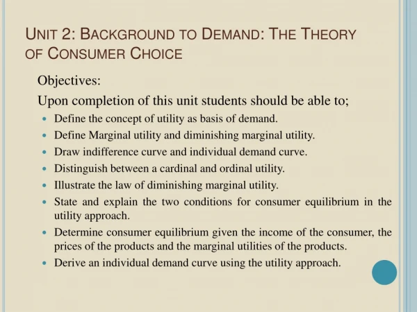
In this chapter, look for the answers to these questions: • How does the budget constraint represent the choices a consumer can afford? • How do indifference curves represent the consumer’s preferences? • What determines how a consumer divides her resources between two goods? • How does the theory of consumer choice explain decisions such as how much a consumer saves, or how much labor she supplies? 1
Introduction Recall one of the Ten Principles from Chapter 1: People face tradeoffs. Buying more of one good leaves less income to buy other goods. Working more hours means more income and more consumption, but less leisure time. Reducing saving allows more consumption today but reduces future consumption. This chapter explores how consumers make choices like these. THE THEORY OF CONSUMER CHOICE
Consumer Theory • Assumes buyers are completely informed about: • Range of products available • Prices of all products • Capacity of products to satisfy • Their income • Requires that consumers can rank all consumption bundles based on the level of satisfaction they would receive from consuming the various bundles
Properties of Consumer Preferences • Completeness • For every pair of consumption bundles, A and B, the consumer can say one of the following: • A is preferred to B • B is preferred to A • The consumer is indifferent between A and B • Transitivity • If A is preferred to B, and B is preferred to C, then Amust be preferred to C • Nonsatiation • More of a good is always preferred to less
Utility • Benefits consumers obtain from goods & services they consume is utility • A utility function shows an individual’s perception of the utility level attained from consuming each conceivable bundle of goods
Marginal Utility • Addition to total utility attributable to the addition of one unit of a good to the current rate of consumption, holding constant the amounts of all other goods consumed
Consumer’s Budget Line • Shows all possible commodity bundles that can be purchased at given prices with a fixed money income
R 120 A 100 F 80 C D B Z N 125 160 250 200 240 Panel B – Changes in price of X Shifting Budget Lines (Figure 5.7) A 100 Quantity of Y Quantity of Y B 200 Quantity of X Quantity of X Panel A – Changes in money income
Utility Maximization • Utility maximization subject to a limited money income occurs at the combination of goods for which the indifference curve is just tangent to the budget line
Utility Maximization • Consumer allocates income so that the marginal utility per dollar spent on each good is the same for all commodities purchased
• A 45 • B • D E • IV R III C • II 15 T I Constrained Utility Maximization (Figure 5.8) 50 Quantity of pizzas 40 30 20 10 0 10 20 30 40 70 80 90 100 50 60 Quantity of burgers
Marginal Rate of Substitution • MRS shows the rate at which one good can be substituted for another while keeping utility constant • Negative of the slope of the indifference curve • Diminishes along the indifference curve as X increases & Y decreases • Ratio of the marginal utilities of the goods
The Budget Constraint: What the Consumer Can Afford Example: Hurley divides his income between two goods:fish and mangos. A “consumption bundle” is a particular combination of the goods, e.g., 40 fish & 300 mangos. Budget constraint: the limit on the consumption bundles that a consumer can afford THE THEORY OF CONSUMER CHOICE
A C T I V E L E A R N I N G 1Budget Constraint Hurley’s income: $1200 Prices: PF = $4 per fish, PM = $1 per mango A. If Hurley spends all his income on fish, how many fish does he buy? B. If Hurley spends all his income on mangos, how many mangos does he buy? C. If Hurley buys 100 fish, how many mangos can he buy? D. Plot each of the bundles from parts A – C on a graph that measures fish on the horizontal axis and mangos on the vertical, connect the dots. 15
B C A A C T I V E L E A R N I N G 1Answers D.Hurley’s budget constraint shows the bundles he can afford. A. $1200/$4= 300fish B. $1200/$1= 1200mangos C. 100fish cost $400,$800 left buys 800mangos Quantity of Mangos Quantity of Fish
C D The Slope of the Budget Constraint From C to D, “rise” =–200 mangos “run” = +50 fish Slope = – 4 Hurley must give up 4 mangos to get one fish. Quantity of Mangos Quantity of Fish THE THEORY OF CONSUMER CHOICE
The Slope of the Budget Constraint The slope of the budget constraint equals the rate at which Hurleycan trade mangos for fish the opportunity cost of fish in terms of mangos the relative price of fish: THE THEORY OF CONSUMER CHOICE
A C T I V E L E A R N I N G 2Budget constraint, continued. Show what happens to Hurley’s budget constraint if: A. His income falls to $800. B. The price of mangos rises to PM = $2 per mango 19
A C T I V E L E A R N I N G 2Answers, part A Now, Hurley can buy $800/$4= 200 fish or$800/$1= 800 mangos or any combination in between. A fall in income shifts the budget constraint down. Quantity of Mangos Quantity of Fish
A C T I V E L E A R N I N G 2Answers, part B Hurley can still buy 300 fish. But now he can only buy $1200/$2 = 600 mangos. Notice: slope is smaller, relative price of fish is now only 2 mangos. An increase in the price of one good pivots the budget constraint inward. Quantity of Mangos Quantity of Fish
B A I1 Preferences: What the Consumer Wants One of Hurley’s indifference curves Indifference curve: shows consumption bundles that give the consumer the same level of satisfaction Quantity of Mangos A, B, and all other bundles on I1 make Hurley equally happy – he is indifferent between them. Quantity of Fish THE THEORY OF CONSUMER CHOICE
B A Four Properties of Indifference Curves One of Hurley’s indifference curves Quantity of Mangos 1.Indifference curves are downward-sloping. If the quantity of fish is reduced, the quantity of mangos must be increased to keep Hurley equally happy. I1 Quantity of Fish THE THEORY OF CONSUMER CHOICE
A I2 I1 D C I0 Four Properties of Indifference Curves A few of Hurley’s indifference curves Quantity of Mangos 2.Higher indifference curves are preferred to lower ones. Hurley prefers every bundle on I2 (like C) to every bundle on I1 (like A). He prefers every bundle on I1 (like A) to every bundle on I0 (like D). Quantity of Fish THE THEORY OF CONSUMER CHOICE
B A C I4 Four Properties of Indifference Curves Hurley’s indifference curves Quantity of Mangos 3.Indifference curves cannot cross. Suppose they did. Hurley should prefer B to C, since B has more of both goods. Yet, Hurley is indifferent between B and C: He likes C as much as A (both are on I4). He likes A as much as B (both are on I1). I1 Quantity of Fish THE THEORY OF CONSUMER CHOICE
Quantity of Mangos B A Quantity of Fish Four Properties of Indifference Curves 4.Indifference curves are bowed inward. Hurley is willing to give up more mangos for a fish if he has few fish (A) than if he has many (B). 6 1 2 I1 1 THE THEORY OF CONSUMER CHOICE
Quantity of Mangos B A Quantity of Fish The Marginal Rate of Substitution MRS = slope of indifference curve Marginal rate of substitution (MRS): the rate at which a consumer is willing to trade one good for another. MRS = 6 Hurley’s MRS is the amount of mangos he would substitute for another fish. 1 MRS = 2 I1 1 MRS falls as you move down along an indifference curve. THE THEORY OF CONSUMER CHOICE
One Extreme Case: Perfect Substitutes Perfect substitutes: two goods with straight-line indifference curves, constant MRS Example: nickels & dimes Consumer is always willing to trade two nickels for one dime. THE THEORY OF CONSUMER CHOICE
Another Extreme Case: Perfect Complements Perfect complements: two goods with right-angle indifference curves Example: Left shoes, right shoes {7 left shoes, 5 right shoes} is just as good as {5 left shoes, 5 right shoes} THE THEORY OF CONSUMER CHOICE
Less Extreme Cases: Close Substitutes and Close Complements Indifference curves for close complements are very bowed Indifference curves for close substitutes are not very bowed Quantity of hot dog buns Quantity of Pepsi Quantity of hot dogs Quantity of Coke
A B C D Optimization: What the Consumer Chooses A is the optimum: the point on the budget constraint that touches the highest possible indifference curve. Quantity of Mangos The optimum is the bundle Hurley most prefers out of all the bundles he can afford. 1200 Hurley prefers B to A, but he cannot afford B. 600 Hurley can afford C and D, but A is on a higher indifference curve. 300 150 Quantity of Fish THE THEORY OF CONSUMER CHOICE
A marginal value of fish (in terms of mangos) price of fish (in terms of mangos) Optimization: What the Consumer Chooses Quantity of Mangos Consumer optimization is another example of “thinking at the margin.” At the optimum, slope of the indifference curve equals slope of the budget constraint: 1200 MRS = PF/PM 600 300 150 Quantity of Fish THE THEORY OF CONSUMER CHOICE
A B The Effects of an Increase in Income Quantity of Mangos An increase in income shifts the budget constraint outward. If both goods are “normal,” Hurley buys more of each. Quantity of Fish THE THEORY OF CONSUMER CHOICE
A C T I V E L E A R N I N G 3Inferior vs. normal goods • An increase in income increases the quantity demanded of normal goods and reduces the quantity demanded of inferior goods. • Suppose fish is a normal good but mangos are an inferior good. • Use a diagram to show the effects of an increase in income on Hurley’s optimal bundle of fish and mangos. 34
A B A C T I V E L E A R N I N G 3Answers Quantity of Mangos If mangos are inferior, the new optimum will contain fewer mangos. Quantity of Fish 35
new optimum 500 600 350 The Effects of a Price Change Quantity of Mangos Initially, PF = $4 PM = $1 1200 initial optimum PF falls to $2 budget constraint rotates outward, Hurley buys more fish and fewer mangos. 600 300 Quantity of Fish 150 THE THEORY OF CONSUMER CHOICE
A fall in the price of fish has two effects on Hurley’s optimal consumption of both goods. Income effectA fall in PF boosts the purchasing power of Hurley’s income, allows him to buy more mangos and more fish. Substitution effect A fall in PF makes mangos more expensive relative to fish, causes Hurley to buy fewer mangos & more fish. Notice: The net effect on mangos is ambiguous. The Income and Substitution Effects THE THEORY OF CONSUMER CHOICE
C B The Income and Substitution Effects Initial optimum at A. PF falls. Substitution effect:from A to B, buy more fish and fewer mangos. Income effect:from B to C, buy more of both goods. Quantity of Mangos In this example, the net effect on mangos is negative. A Quantity of Fish THE THEORY OF CONSUMER CHOICE
Substitution & Income Effects • Substitution effect • Change in consumption of a good after a change in its price, when the consumer is forced by a change in money income to consume at some point on the original indifference curve • Income effect • Change in consumption of a good resulting strictly from a change in purchasing power
Total effect of price decrease Income effect Substitution effect Total effect of price decrease Income effect Substitution effect + = + = 9 + 4 = 5 3 + (-2) = 5 Income & Substitution Effects: A Decrease in Px(Figure 5.12)
Application 1: Giffen Goods Do all goods obey the Law of Demand? Suppose the goods are potatoes and meat,and potatoes are an inferior good. If price of potatoes rises, substitution effect: buy less potatoes income effect: buy more potatoes If income effect > substitution effect, then potatoes are a Giffen good, a good for which an increase in price raises the quantity demanded. THE THEORY OF CONSUMER CHOICE
Application 1: Giffen Goods THE THEORY OF CONSUMER CHOICE
Application 2: Wages and Labor Supply Budget constraint Shows a person’s tradeoff between consumption and leisure. Depends on how much time she has to divide between leisure and working. The relative price of an hour of leisure is the amount of consumption she could buy with an hour’s wages. Indifference curve Shows “bundles” of consumption and leisure that give her the same level of satisfaction. THE THEORY OF CONSUMER CHOICE
Application 2: Wages and Labor Supply At the optimum, the MRS between leisure and consumption equals the wage. THE THEORY OF CONSUMER CHOICE
Application 2: Wages and Labor Supply An increase in the wage has two effects on the optimal quantity of labor supplied. Substitution effect(SE): A higher wage makes leisure more expensive relative to consumption. The person chooses less leisure, i.e., increases quantity of labor supplied. Income effect (IE): With a higher wage, she can afford more of both “goods.” She chooses more leisure, i.e., reduces quantity of labor supplied. THE THEORY OF CONSUMER CHOICE
Application 3: Interest Rates and Saving A person lives for two periods. Period 1: young, works, earns $100,000 consumption = $100,000 minus amount saved Period 2: old, retired consumption = saving from Period 1 plus interest earned on saving The interest rate determinesthe relative price of consumption when young in terms of consumption when old. THE THEORY OF CONSUMER CHOICE
Application 3: Interest Rates and Saving Budget constraint shown is for 10% interest rate. At the optimum, the MRS between current and future consumption equals the interest rate. THE THEORY OF CONSUMER CHOICE