Download

1 / 35
350 likes | 504 Views
Broadband PLC Radiation from a Power Line with Sag. Nan Maung, SURE 2006 SURE Advisor: Dr. Xiao-Bang Xu. OBJECTIVE. To model a radiating Catenary Line Source (Eg. An Outdoor wire with sag) Understand Physical Interpretation of Mathematical Models

E N D
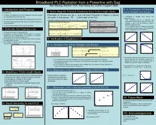
Broadband PLC Radiation from a Power Line with Sag Nan Maung, SURE 2006 SURE Advisor: Dr. Xiao-Bang Xu
OBJECTIVE • To model a radiating Catenary Line Source (Eg. An Outdoor wire with sag) • Understand Physical Interpretation of Mathematical Models • To use theoretical knowledge to test whether Model and Numerical Solutions created are Physically Reasonable
INTENDED MODELCatenary Wire Modeled by Finite-Length Dipoles
INTENDED MODEL • Number of dipoles • Dipole Midpoints
THEORY Solutions are derived based on: • Superposition • Helmholtz Equation • Fourier Transform Techniques • Sommerfeld Radiation Conditions
ANALYSIS & VERIFICATION • Solution must make Physical sense • Intermediate (simpler) Models used for verification • A Straight Line Source • A Hertzian Dipole • Compare Solution derived for Catenary to Line Source • Hertzian Dipole is used as basis for model of Finite-Length Dipole
METHOD OF SOLUTION(General) • Boundary Value Problem • Define Source Type • Derive Helmholtz Equation for Vector Magnetic Potential • Forward Fourier Transform • Find Solution in Spectral Domain (SD) • TD Solution must satisfy Sommerfeld Radiation Condition • Inverse Fourier Transform • IFT Integrals must be convergent
A Straight-Line Source • Located in upper Half-Space above Media Interface at z = 0
Predicted behavior of SolutionsBased on Physical Interpretation • First term in is due to an infinite line source in homogeneous medium • First term in is due to image of the line source in a PEC plane at the boundary • Second term in is correction for the fact that a PEC plane does not faithfully model the media interface and Region b • The correction term should decrease if the dielectric properties of Medium b are allowed to approach those of Medium a
NUMERICAL RESULTS & SOLUTION CHECK Real and imaginary parts of Correction Integral vs. Relative Dielectric of Medium b Observed at z=15
NUMERICAL RESULTS & SOLUTION CHECK Real and Imaginary parts of Correction Integral vs. Relative Dielectric of Medium b Observed at z = 7
A Hertzian Dipole • Source Definition • Helmholtz Equation • Boundary Conditions • Dyadic Green’s Function • F.T. Solution for Dyadic Elements • Sommerfeld Integrals
PHYSICAL INTERPRETATION OF • First term is potential due to dipole in Infinite Homogeneous Medium • Second Term represents Reflection (Medium Interface Effect) • Second Term should decrease if dielectric properties of Medium b to approach those of Medium a • Potential should decay away from the wire
NUMERICAL RESULTS & SOLUTION BEHAVIOR Media Interface Effect for various Medium b Relative Dielectric
NUMERICAL RESULTS & SOLUTION BEHAVIOR Magnitude of Potential for Dipole at z’=10 • LEFT: below z’ • RIGHT: above z’
A Finite-Length Dipole • Source Definition • Helmholtz Equation • Boundary Conditions • Dyadic Green’s Function • F.T. Solution for Dyadic Elements • Sommerfeld Integrals
Finite-Length Dipole Linear Approximation • Assume q small (H >> L) • Approximate by a Hertzian dipole at midpoint • Multiplied by length L of dipole
BEHAVIOR OF SOLUTIONS • How does deviation from a straight line (amount of sag) affect potentials above and below the Catenary line • Compare to potentials created by straight line source
NUMERICAL RESULT Imaginary part of x-directed potential at z=7 • Potential due to line source • = 1.4839e-007 +1.9810e-007i
NUMERICAL RESULT Imaginary part of x-directed potential at z=7 • Potential due to line source • = 1.4839e-007 +1.9810e-007i
COMPARISON OF CATENARY MODELLED BY DIPOLES TO STRAIGHT LINE • Real and Imaginary parts of two potentials are observed separately • As amount of Sag is decreased: • Re( ) Re( ) • Im( ) Im ( )* • At field points below the two sources
FUTURE WORK • Linear Approximation of Finite Length Dipole (H>>l) • Made due to time constraint • A better approximation or Line Integral
FUTURE WORK • Earth is assumed Lossless Dielectric • Could also be studied as Lossy Dielectric • Better understanding of how to compare a problem with 2-D Geometry (Infinite Straight Line) to 3-D Geometry (Dipole)
FUTURE WORK • Straight line originally analyzed with orientation shown • Potentials were z-directed • Coordinate system had to be changed for comparison with Catenary line
ACKNOWLEDGEMENTS • Dr. Xiao-Bang Xu, SURE Advisor • Dr. Daniel L. Noneaker, SURE Program Director • National Science Foundation • 2006 SURE Students and Graduate Assistant Karsten Lowe