Download
1 / 18
180 likes | 371 Views
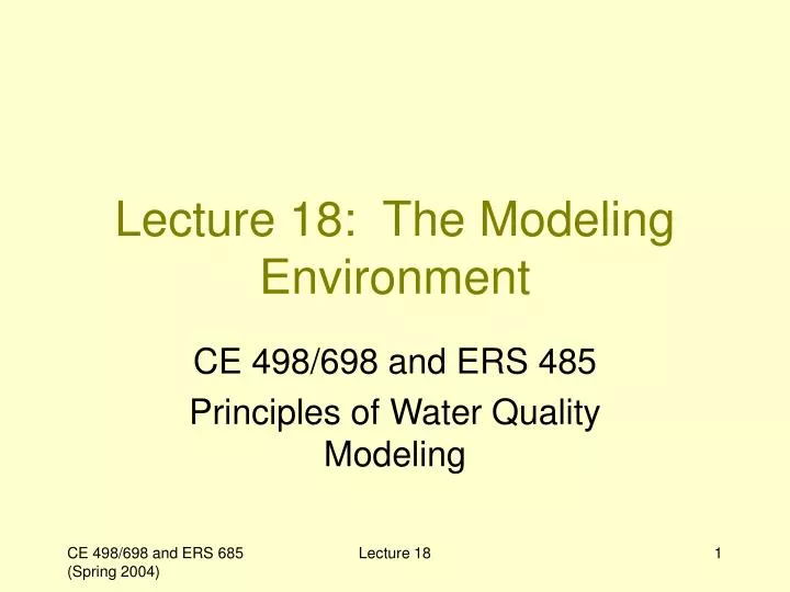
Lecture 18: The Modeling Environment. CE 498/698 and ERS 485 Principles of Water Quality Modeling. The modeling environment. Models are an idealized formulation that represents the response of a physical system to external stimuli (p. 10)

E N D
Lecture 18: The Modeling Environment CE 498/698 and ERS 485 Principles of Water Quality Modeling Lecture 18
The modeling environment • Models are an idealized formulation that represents the response of a physical system to external stimuli (p. 10) • Models are tools that are part of an overall management process Lecture 18
Data collection Management (or scientific) objectives, options, constraints Make management decisions Model development and application Lecture 18
Rules of modeling • RULE 1: We cannot model reality • We have to make assumptions • DOCUMENT!!!! • RULE 2: Real world has less precision than modeling Lecture 18
Precision vs. accuracy • Precision • Number of decimal places • Spread of repeated computations • Accuracy • Error between computed or measured value and true value error of estimate = field error + model error Lecture 18
Difference = 10.056 deg C Location B Location A The problem with precise models… we get more precision from model than is real Model says… Lecture 18
Figure 18.1 (Chapra 1997) Lecture 18
Modeling in management process • Problem specification • Do we need to model? • Model selection • Who will the users be? • What kind of data is available? • General model or specific? • Use existing model or develop a new one? Lecture 18
Modeling in management process • Model development • Develop/modify code • Input data • Determine numerical approach • model resolution • Timestep • Spatial size Lecture 18
Figure 18.9 (Chapra 1997) Lecture 18
Modeling in management process • Model development • Develop/modify code • Input data • Determine numerical approach • model resolution • Timestep • Spatial size • Matter Lecture 18
Modeling in management process • Preliminary application and calibration Figure 18.3 (Chapra 1997) Lecture 18
Modeling in management process • Preliminary application and calibration • Adjust parameters • Adjust input data (where appropriate) • Compare model predictions with measured Lecture 18
Calibration measures • Chapra: minimize sum of squares of residuals where cp,i= model prediction for i cm,i = measured value for i smallest sum is best! Lecture 18
0 ≤r2 ≤ 1 Calibration measures • Chapra: minimize sum of squares of residuals • R-squared: how much of the variability in the observed data is explained by the predicted data Lecture 18
Calibration measures • Average absolute error • Root mean squared error Calibration is a KEY process! Lecture 18
Modeling in management process • Model confirmation (validation) • Use an independent data set for measured values • Use same parameters/coefficients, same methods of estimating data • Does model still work???? Lecture 18
Modeling in management process • Management application • Verification • Sensitivity analysis Lecture 18