Download
1 / 99
1.01k likes | 1.15k Views
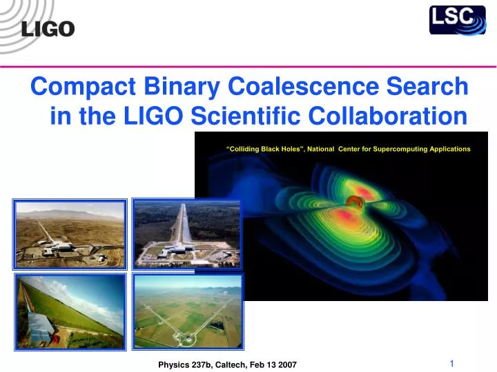
Compact Binary Coalescence Search in the LIGO Scientific Collaboration. “Colliding Black Holes”, National Center for Supercomputing Applications. Outline. The signal we are trying to detect How far we can detect How many sources we can detect establishing an upper limit on the sources

E N D
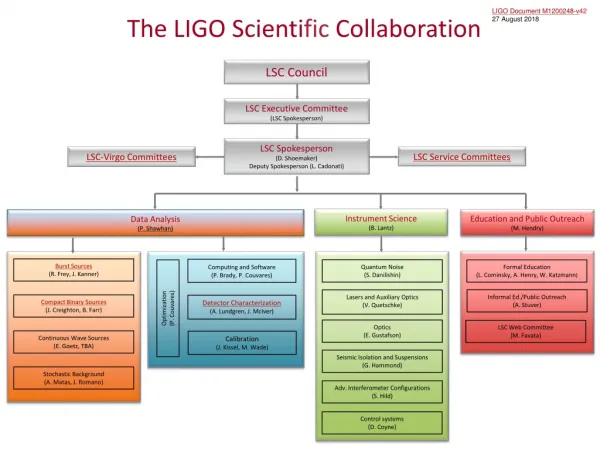
Compact Binary Coalescence Search in the LIGO Scientific Collaboration “Colliding Black Holes”, National Center for Supercomputing Applications
Outline • The signal we are trying to detect • How far we can detect • How many sources we can detect • establishing an upper limit on the sources • How to suppress noise • The analysis pipeline • detection confidence • parameter estimation • software
Compact Binary Coalescence • LIGO, GEO, Virgo and TAMA search for GW signals from the last few minutes of coalescence of a compact binary system with component masses between ~1 and ~100 solar masses, within a few 100 Mpc of the Earth. • Inspiral Merger Ringdown
Inspiral signal in t-f • time-frequency spectrogram q-scan
Signal parameters • For non-spinning binaries, we have 7 parameters that affect the amplitude of the signal but not its general form (“extrinsic parameters”): • source sky location: (ra, dec) or, in detector frame, (,) • source physical distance r (sometimes written d) • orientation of orbital plane: inclination angle and polarization • orbital phase at coalescence 0, and time of coalescence tc • And two parameters that do affect the form of the signal (the evolution of its amplitude and phase – “intrinsic parameters”): • (m1, m2), • or chirp mass Mc = Mtot (2/5) and symmetric mass ratio = m1 m2 / mtot2 • or total mass Mtot = m1 + m2 and reduced mass Mtot
Signal parameters • For spinning binaries, add three more parameters each for the spin vector of each component relative to the orbital plane of the binary (total: 15 parameters). • Late in the inspiral, the orbits have circularized due to radiation back-reaction, but early on, orbits are in general elliptical: add initial ellipticity , and two angles for the orientation of the semi-major axis. • Current LIGO searches use non-spinning templates; even in a 2-D intrinsic parameter space, we have tens of thousands of templates. • Much effort is now going in to searches using spinning templates, but tricks are required to make the problem computationally manageable. • BCV and BCV-spin “detection template” families • “Physical template” family developed by Pan et el
Signal templates in frequency space, in Stationary Phase Approximation (SPA) Normalization: Effective distance:
Evolution of Binary System • This is just the inspiral phase, well predicted by post-Newtonian PT, expanding in x ~ (v/c)2 • What about the merger and ringdown? Lots of GWs! • In the last few years, breakthroughs in numerical relativity are giving us ~ quantitative results on these phases!
Evolution of amplitude and frequency through merger and ringdown comparison of analytic and numerical coalescing binary waveforms: nonspinning case; arXiv:0704.1964v2 (2007), Pan, Buonanno, et al
Energy radiated through IMR Inspiral, merger and ring-down of equal-mass black-hole binaries Buonanno, Cook, Pretorius, arXiv:gr-qc/0610122v2 2007
Inspiral-Merger-Ringdown • NR waveforms covering the full parameter space are still under development, and trust in their veracity is still pending • Generation of NR waveforms for a given set of parameters is slow, and generating families of templates covering the intrinsic parameter space would take too long • Much work is in progress to match NR waveforms with analytical models (PN, EOB, ringdowns…) to enable “hybrid” IMR waveforms for template banks and testing of detection pipelines • Meanwhile, the LSC has chosen to search for inspiral, merger, and ringdown phases in separate search pipelines • Inspiral and ringdown searches use matched filtering with template banks • merger phase is the “burst” search • Bringing them together in “IMR” coincident trigger analyses is only now under development, and not yet in place. • today, focus on inspiral search analysis.
Science Runs A Measure of Progress Milky Way Virgo Cluster Andromeda NN Binary Inspiral Range 4/02: E8 ~ 5 kpc 10/02: S1 ~ 100 kpc 4/03: S2 ~ 0.9Mpc 11:03: S3 ~ 3 Mpc Design~ 18 Mpc
Best Performance to Date …. Current: all three detectors are at design sensitivity from ~ 60 Hz up! h ~ 210-23 /rtHz x ~ 8 10-20 m/rtHz
Inspiral horizon distance • Much of the accumulated SNR is in the last few cycles, so the horizon distance depends on where we (our templates) take the inspiral phase to end (ie, at what component separation r or velocity v/c = (GM/c2r)(1/2) : • Innermost stable circular orbit: r = 6M • Equivalent-one-body (EOB) “light-ring” orbit: r = 2.8M(circular orbit of photons in the Schwarzschild metric) • Where you think the perturbation expansion in v/c breaks down • Geometric units: Rsun = GMsun/c2 = 1477 m; Tsun = GMsun/c3 = 4.9 µs • GW Frequency at r = bM: fGW = 2 forb = (GMr3)(1/2)/ (Kepler) = c3/(GMb(3/2))
Signal templates in frequency space, in Stationary Phase Approximation (SPA) Normalization: Effective distance:
Inspiral Horizon Distance Distance to optimally located and oriented1.4,1.4 solar mass BNS, at SNR = 8using templates that end at ISCO S3 Science Run Oct 31, 2003 - Jan 9, 2004
Inspiral Horizon Distance Distance to optimally oriented 1.4,1.4 solar mass BNS at SNR = 8 S4 Science Run Feb 22, 2005 - March 23, 2005
Inspiral Horizon Distance Distance to optimally oriented 1.4,1.4 solar mass BNS at SNR = 8 First Year S5 Science Run Nov 4, 2005 - Nov 14, 2006
Inspiral horizon distance • SNR depends strongly on the ending frequency (relative to the noise curve “bucket”, which in turn depends strongly on the mass of the system
Horizon Distance vs. Mass – S5 Binary Neutron Stars
Inspiral duration • “In-band” duration of inspiral, in seconds and in cycles, also depends strongly on mass: t ~ (5MTsun/256) (MTsun flow)-8/3 Higher-order effects!
Inspiral duration • Initial LIGO (flow~ 40 Hz): BNS ~ 15 s; BBH 100Msun : a few msec, < 3 cycles – burst! • Advanced LIGO (flow~ 15 Hz): BNS ~ 300 s or more, requiring new filtering techniques – MultiBandTemplateApprox MBTA) Higher-order effects!
Matched Filtering • Assume the signal we are searching for is known, up to unknown arrival time, constant phase and amplitude • Construct matched filter statistic for this signal
Matched Filtering • Choose templates to be normalized to strain at 1 Mpc • Cutoff flow is determined by detector noise curve, fmax by template • Effective distance to signal is given by
Triggers: threshold on peaks in the matched filter output time series
Mismatch • What if the template is incorrect? • Loss in signal to noise ratio is given by the mismatch
Mismatch and Event Rate • Any mismatch between signal and template reduces the distance to which we can detect inspiral signals • Loss in signal-to-noise ratio is loss in detector range • Loss in event rate = (Loss in range)3 • We must be careful that the mismatch between the signal and our templates does not unacceptably reduce our rate
Inspiral Template Banks • To search for signals in the mass region of interest, we must construct a template bank • Lay down grid of templates so that loss in SNR between signal in space and nearest template is no greater than ~ 3%
Overview of S1 - S4 Searches 40.0 BBH Search S2 - S4 Detection Templates Ringdowns S4 3.0 BNS S1-S4 PN NS/BH S3 Spin is important Detection Templates 1.0 1.0 3.0 40.0 100.0 150.0
Overview of S5 Searches 40.0 Ringdowns Burst EOB 3.0 PN Templates 1.0 1.0 3.0 40.0 100.0 150.0
Astrophysical source distribution • Our primary goal is to detect GWs from compact binary coalescences and study the properties of individual systems. • Once we observe many such systems, we wish to constrain the astrophysical source distribution. • Until we make detections, we wish to bound the CBC rate in the universe. • To do this, we need a model of the astrophysical source distribution: spatial distribution and mass distribution.
Astrophysical source distribution • Population synthesis provides limited guidance: • models of stellar formation and evolution, and the formation and evolution of compact binaries, contain many uncertainties. • The only real observational constraints on these models come from the handful of relativistic pulsar binary systems (BNS) observed in our galaxy. • There are essentially no observational constraints on systems containing 10 or 100 solar mass black holes; yet these are some of the most promising sources for LIGO! • The astrophysical distribution of CB mass beyond BNS is hardly constrained at all: we choose to measure the rate as a function of CB total mass.
Binary Neutron Star Inspiral Rate Estimates • Base on observed systems, or on population synthesis Monte Carlo • Kalogera et al., 2004 ApJ 601, L179 • Statistical analysis of the 3 known systems with “short” merger times • Simulate population of these 3 types • Account for survey selection effects • For reference population model: • (Bayesian 95% confidence) • Milky Way rate: 180+477–144 per Myr • LIGO design: 0.015–0.275 per year • Advanced LIGO: 80–1500 per year • Binary black holes, BH-NS:No known systems; must Monte Carlo
Source Distribution Beyond the MW • Pop.synth. and general astrophysical wisdom says: compact binary systems exist in galaxies. Specifically, “young” galaxies with lots of star formation (spirals); less so for older galaxies like ellipticals. • Logic (as far as I understand it): CBC’s represent (one path for) the death of stars; in a steady-state situation, it should be proportional to the stellar birth rate. • Star-birth involves young, massive, hot stars, emitting blue light. Hence, the CBC rate is, in this simplest model, proportional to blue-light luminosity (Phinney, 1991).
Astrophysical source distribution • This can’t be strictly true: the time scale for coalescence can be of the same order as the age of the universe. Some component of the CBC rate must be proportional to the total number of stars (mass), not the stellar birth rate. Older galaxies (eg, ellipticals) must contribute. • Nonetheless, we stick with the simplest model: CBC rate is proportional to blue-light luminosity. • Our only astrophysical constraints on CBC rate are from BNS progenitors in the Milky Way, so we can estimate the rate per Milky Way Equivalent Galaxy (MWEG).
Astrophysical source distribution • Problem: we don’t know the blue-light luminosity of the MW very well! It is directly measurable for our sun (Lsun-BL) and for other galaxies, only estimated for MW (MWEG ~ 1.5 – 2.0 1010 Lsun-BL with a best estimate of 1.7 1010 Lsun-BL = 1.7 L10). • In LIGO S2, we were mainly sensitive to the MW, so normalizing the astrophysical rate to MWEG was appropriate. • By S3 we are touching M31 and beyond. But although the MW is overdense with sources, the empty space between the MW and M31, and between out local cluster and the Virgo cluster, is underdense. • Fortunately, it’s not distances that matter so much as effective distance: sources that are not optimally located (detector zenith) or oriented (face-on) have a correspondingly larger effective distance that is always larger than the physical distance. This smooths out the fluctuations in source density.
Astrophysical source distribution • By S4 and S5, our source population is dominated by galaxies beyond the MW, so we have switched to normalizing the CBC rate to L10 ~ 1/1.7 MWEG. • Beyond about 20 Mpc, the source density is more-or-less uniform at ~ 0.01 L10 per Mpc3 , and number of sources grows like horizon distance cubed. • The LSC now quote rate upper limits in units of [ 1 / L10 / yr ]. • Some of the most significant systematic errors associated with the search upper limits are due to uncertainties in the astrophysical source distribution! Nearby source distances and luminosities. • By S5, we will be well into the uniform regime where we only need to know = 0.01 L10 / Mpc3 with, say, 10% error.
Loudest event statistic • This is a novel, but rather natural method for establishing a Bayesian confidence interval or upper limit on the rate for a process characterized by events with a “loudness” (eg, coincident inspiral triggers characterized by a combined SNR). • “Loudness” measures how signal-like an event is: loud events are more likely to be signal than noise (background). It is also referred to as a “detection statistic” . • It can be more complicated than an SNR; for example, it could contain information about how “signal-like” the signal is, eg, from a chisq test.
Loudest event statistic • Traditionally, one sets a fixed threshold on event loudness *; louder events are called “signal” (although they may be contaminated by background) and less loud events are ignored as background. • One then assumes a certain parent (source) distribution, and uses Monte Carlo simulation to estimate the probability that an event drawn from that distribution would be louder than the threshold (the search efficiency). • The confidence interval or upper limit on the rate is then established by combining the number of events observed above threshold, the estimated background, and the efficiency for detecting an event from the assumed source distribution. Eg, Rate = (Nobs – Nbcknd)/(efficiency * time). • In absence of detection (and background), with no events observed, Rate < -ln(1-CL)/(efficiency * time) = 2.3/(eff*time) @ 90% CL.
Loudest event statistic • For Initial LIGO, this traditional procedure is dangerous: • The expected detection rate is below our current sensitivity (we expect to see less than one event in S5). • Our background rate is difficult to determine, because our detectors are novel and not very well understood, and glitchier than we would like. • The stakes are high! We don’t want to declare a detection just because we’ve accidentally underestimated our background. • The traditional procedure has already bitten us: The LIGO burst search established a fixed threshold where we believed that the false alarm rate was << 1 per observation time. Then we observed an event above that threshold in S2! It was caused by acoustic pickup from a low-flying airplane. • Moral: setting a priori fixed thresholds can be dangerous!
Loudest event statistic • Better approach: set a threshold just above the loudest observed event. • Then, by definition, there will be no signal events to sweat over! • Set a (conservative) upper limit on the rate, based on the efficiency for detecting events from the source distribution with loudness above that threshold. • If we have true signal below our threshold, the true rate should be below the resulting upper limit (with a specified statistical confidence); the upper limit is “conservative”. • We can still detect! Examine each of the loudest events in the search (all below the loudest event threshold), and use a variety of tests (the “detection checklist”) to establish “detection confidence”. S4 PBH S4 BBH S4 BNS Loudest event
Loudest event statistic • We wish to measure the rate R of events/yr/L10 • Predicted number of events expected above a given detection statistic threshold (eg, that of the loudest observed event): Np = R·T·CL(*) • We can compute an estimate of the cumulative luminosity CL (in units of L10) to which we are sensitive. Crudely, CL = L10· (4/3) D(*)3where * is our SNR (or detection statistic) thresholdand D is the (average over sky location and orientation) distance below which we can detect a signal with detection statistic < *. • This will depend on the signal parameters (mainly, chirp mass). • More precisely, we perform a convolution integral over our source density model (as a function of physical distance) and our detection efficiency vs distance (as measured using simulated signal injections, run through the full detection pipeline).
Loudest event statistic • Detection efficiency is a gentle function of physical distance; but it’s a sharper function of effective distance. More efficient to use that. • But effective distance depends on the detector; it’s different at LHO and LLO. Need to do the convolution in 2D for LIGO-only analysis. ~
Loudest event statistic • Predicted number of events expected above a given detection statistic threshold (eg, that of the loudest observed event): Np = R·T·CL(m ) • Probability of observing no events above x* (in absence of background) is P(m) = exp(-Np) • If we estimate that the background has a probability Pb(m) of having (at least) one event above x*, thenP(m) = Pb(m) ·exp(-Np(m)) • Applying a Bayesian analysis with uniform prior on R, we can turn this into a probability distribution for R, and set an upper limit (at xome confidence level) on R, R*:
Loudest event statistic • Here, in the presence of background, measures the lilelihood that the loudest event is real, as opposed to background: • Limiting cases:loudest event is unlikely to be bg:loudest event is most likely bg: • is pretty small for the S4 searches.