Download

1 / 40
400 likes | 525 Views
Loop Transformations and Locality . Agenda. Introduction Loop Transformations Affine Transform Theory. Memory Hierarchy. CPU. C. C. Cache. Memory. Cache Locality. Suppose array A has column-major layout. for i = 1, 100 for j = 1, 200 A[i, j] = A[i, j] + 3 end_for end_for.

E N D
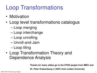
Agenda • Introduction • Loop Transformations • Affine Transform Theory
Memory Hierarchy CPU C C Cache Memory
Cache Locality • Suppose array A has column-major layout for i = 1, 100 for j = 1, 200 A[i, j] = A[i, j] + 3 end_for end_for • Loop nest has poor spatial cache locality.
Loop Interchange • Suppose array A has column-major layout for j = 1, 200 for i = 1, 100 A[i, j] = A[i, j] + 3 end_for end_for for i = 1, 100 for j = 1, 200 A[i, j] = A[i, j] + 3 end_for end_for • New loop nest has better spatial cache locality.
Interchange Loops? for i = 2, 100 for j = 1, 200 A[i, j] = A[i-1, j+1]+3 end_for end_for j i • e.g. dependence from (3,3) to (4,2)
Dependence Vectors • Distance vector (1,-1) = (4,2)-(3,3) • Direction vector (+, -) from the signs of distance vector • Loop interchange is not legal if there exists dependence (+, -) j i
Agenda • Introduction • Loop Transformations • Affine Transform Theory
Loop Fusion for i = 1, 1000 A[i] = B[i] + 3 end_for for j = 1, 1000 C[j] = A[j] + 5 end_for for i = 1, 1000 A[i] = B[i] + 3 C[i] = A[i] + 5 end_for • Better reuse between A[i] and A[i]
Loop Distribution for i = 1, 1000 A[i] = A[i-1] + 3 end_for for i = 1, 1000 C[i] = B[i] + 5 end_for for i = 1, 1000 A[i] = A[i-1] + 3 C[i] = B[i] + 5 end_for • 2nd loop is parallel
Register Blocking for j = 1, 2*m, 2 for i = 1, 2*n, 2 A[i, j] = A[i-1,j] + A[i-1,j-1] A[i, j+1] = A[i-1,j+1] + A[i-1,j] A[i+1, j] = A[i, j] + A[i, j-1] A[i+1, j+1] = A[i, j+1] + A[i, j] end_for end_for for j = 1, 2*m for i = 1, 2*n A[i, j] = A[i-1, j] + A[i-1, j-1] end_for end_for • Better reuse between A[i,j] and A[i,j]
Virtual Register Allocation for j = 1, 2*M, 2 for i = 1, 2*N, 2 r1 = A[i-1,j] r2 = r1 + A[i-1,j-1] A[i, j] = r2 r3 = A[i-1,j+1] + r1 A[i, j+1] = r3 A[i+1, j] = r2 + A[i, j-1] A[i+1, j+1] = r3 + r2 end_for end_for • Memory operations reduced to register load/store • 8MN loads to 4MN loads
Scalar Replacement t1 = A[1] for i = 2, N+1 = t1 + 1 t1 = A[i] = t1 end_for for i = 2, N+1 = A[i-1]+1 A[i] = end_for • Eliminate loads and stores for array references
Unroll-and-Jam for j = 1, 2*M, 2 for i = 1, N A[i, j]=A[i-1,j]+A[i-1,j-1] A[i, j+1]=A[i-1,j+1]+A[i-1,j] end_for end_for for j = 1, 2*M for i = 1, N A[i, j] = A[i-1, j] + A[i-1, j-1] end_for end_for • Expose more opportunity for scalar replacement
Large Arrays • Suppose arrays A and B have row-major layout for i = 1, 1000 for j = 1, 1000 A[i, j] = A[i, j] + B[j, i] end_for end_for • B has poor cache locality. • Loop interchange will not help.
Loop Blocking for v = 1, 1000, 20 for u = 1, 1000, 20 for j = v, v+19 for i = u, u+19 A[i, j] = A[i, j] + B[j, i] end_for end_for end_for end_for • Access to small blocks of the arrays has good cache locality.
Loop Unrolling for ILP for I = 1, 10, 2 a[i] = b[i]; *p = … a[i+1] = b[i+1]; *p = … end_for for i = 1, 10 a[i] = b[i]; *p = ... end_for • Large scheduling regions. Fewer dynamic branches • Increased code size
Agenda • Introduction • Loop Transformations • Affine Transform Theory
Objective • Unify a large class of program transformations. • Example: float Z[100]; for i = 0, 9 Z[i+10] = Z[i]; end_for
Iteration Space • A d-deep loop nest has d index variables, and is modeled by a d-dimensional space. The space of iterations is bounded by the lower and upper bounds of the loop indices. • Iteration space i = 0,1, …9 for i = 0, 9 Z[i+10] = Z[i]; end_for
Matrix Formulation • The iterations in a d-deep loop nest can be represented mathematically as • Z is the set of integers • B is a d x d integer matrix • b is an integer vector of length d, and • 0 is a vector of d 0’s.
Example for i = 0, 5 for j = i, 7 Z[j,i] = 0; • E.g. the 3rd row –i+j ≥ 0 is from the lower bound j ≥ i for loop j.
Symbolic Constants for i = 0, n Z[i] = 0; • E.g. the 1st row –i+n ≥ 0 is from the upper bound i ≤ n.
Data Space • An n-dimensional array is modeled by an n-dimensional space. The space is bounded by the array bounds. • Data space a = 0,1, …99 float Z[100] for i = 0, 9 Z[i+10] = Z[i]; end_for
Processor Space • Initially assume unbounded number of virtual processors (vp1, vp2, …) organized in a multi-dimensional space. • (iteration 1, vp1), (iteration 2, vp2),… • After parallelization, map to physical processors (p1, p2). • (vp1, p1), (vp2, p2), (vp3, p1), (vp4, p2),…
Affine Array Index Function • Each array access in the code specifies a mapping from an iteration in the iteration space to an array element in the data space • Both i+10 and i are affine. float Z[100] for i = 0, 9 Z[i+10] = Z[i]; end_for
Array Affine Access • The bounds of the loop are expressed as affine expressions of the surrounding loop variables and symbolic constants, and • The index for each dimension of the array is also an affine expression of surrounding loop variables and symbolic constants
Matrix Formulation • Array access maps a vector i within the bounds to array element location Fi+f. • E.g. access X[i-1] in loop nest i,j
Affine Partitioning • An affine function to assign iterations in an iteration space to processors in the processor space. • E.g. iteration i to processor 10-i. float Z[100] for i = 0, 9 Z[i+10] = Z[i]; end_for
Data Access Region • An affine function to assign iterations in an iteration space to processors in the processor space. • Region for Z[i+10] is {a | 10 ≤ a ≤ 20}. float Z[100] for i = 0, 9 Z[i+10] = Z[i]; end_for
Data Dependences • Solution to linear constraints as shown in the last lecture. • There exist ir, iw, such that • 0 ≤ ir, iw ≤9, • iw + 10 = ir float Z[100] for i = 0, 9 Z[i+10] = Z[i]; end_for
Affine Transform j v i u
Locality Optimization for u = 1, 200 for v = 1, 100 A[v,u] = A[v,u]+ 3 end_for end_for for i = 1, 100 for j = 1, 200 A[i, j] = A[i, j] + 3 end_for end_for
Old Iteration Space for i = 1, 100 for j = 1, 200 A[i, j] = A[i, j] + 3 end_for end_for
New Iteration Space for u = 1, 200 for v = 1, 100 A[v,u] = A[v,u]+ 3 end_for end_for
Old Array Accesses for i = 1, 100 for j = 1, 200 A[i, j] = A[i, j] + 3 end_for end_for
New Array Accesses for u = 1, 200 for v = 1, 100 A[v,u] = A[v,u]+ 3 end_for end_for
Interchange Loops? for i = 2, 1000 for j = 1, 1000 A[i, j] = A[i-1, j+1]+3 end_for end_for j i • e.g. dependence vector dold = (1,-1)
Interchange Loops? • A transformation is legal, if the new dependence is lexicographically positive, i.e. the leading non-zero in the dependence vector is positive.
Summary • Locality Optimizations • Loop Transformations • Affine Transform Theory