Floating point numbers
This document explores the concept of computable real numbers, emphasizing their representation through decimal expansions and their limitations. The text discusses finite means of computation as posited by A. M. Turing, showing how decimal approximations improve with additional digits. It examines the significance of transcendental numbers and their inability to have finite representations. Furthermore, it analyzes various numerical storage methods, such as string representation and binary-coded decimal, while also evaluating the trade-offs in precision and performance in systems like Mathematica and Octave.

Floating point numbers
E N D
Presentation Transcript
Computable reals • “computable numbers may be described briefly as the real numbers whose expressions as a decimal are calculable by finite means.”(A. M. Turing, On Computable Numbers with an Application to the Entschiedungsproblem, Proc. London Mathematical Soc., Ser. 2 , Vol 42, pages 230-265, 1936-7.)
Look first at decimal reals • A real number may be approximated by a decimal expansion with a determinate decimal point. • As more digits are added to the decimal expansion the precision rises. • Any effective calculation is always finite – if it were not then the calculation would go on for ever. • There is thus a limit to the precision that the reals can be represented as.
Transcendental numbers • In principle, transcendental numbers such as Pi or root 2 have no finite representation • We are always dealing with approximations to them. • We can still treat Pi as a real rather than a rational because there is always an algorithmic step by which we can add another digit to its expansion.
32 34 39 2E 37 35 First solution • Store the numbers in memory just as they are printed as a string of characters. • 249.75 Would be stored as 6 bytes as shown below Note that decimal numbers are in the range 30H to 39H as ascii codes Full stop char Char for 3
Implications • The number strings can be of variable length. • This allows arbitrary precision. • This representation is used in systems like Mathematica which requires very high accuracy.
Example with Mathematica • 5! • Out[1]=120 • In[2]:=10! • Out[2]=3628800 • In[3]:=50! • Out[3]=30414093201713378043612608166064768844377641568960512000000000000
Decimal byte arithmetic “9”+ “8”= “17” decimal • 39H+38H=71H hexadecimal ascii • 57+56=113 decimal ascii • Adjust by taking 30H=48 away -> 41H=65 • If greater than “9”=39H=57 take away 10=0AH and carry 1 • Thus 41H-0Ah = 65-10=55=37H so the answer would be 31H,37H = “17”
32 34 39 2E 37 35 Representing variables • Variables are represented as pointers to character strings in this system • A=249.75 A
Advantages • Arbitrarily precise • Needs no special hardware Disadvantages • Slow • Needs complex memory management
Binary Coded Decimal (BCD) or Calculator style floating point • Note that 249.75 can be represented as 2.4975 x 10² • Store this 2 digits to a byte to fixed precision as follows mantissa exponent 24 97 50 02 Each digit uses 4 bits 32 bits overall
Normalise Convert N to format with one digit in front of the decimal point as follows: • If N>10 then Whilst N>10 divide by 10 and add 1 to the exponent • Else whilst N<1 multiply by 10 and decrement the exponent
Add floating point • Denormalise smaller number so that exponents equal • Perform addition • Renormalise Eg 949.75 + 52.0 = 1002.75 9.49750 E02 → 9.49750 E02 5.20000 E01 →0.52000 E02 + 10.02750 E02 → 1.00275 E03
Note loss of accuracy Compare Octave which uses floating point numbers with Mathematica which uses full precision arithmetic • Octave floating point gives only 5 figure accuracy Mathematica 5! Out[1]=120 10! Out[2]=3628800 50! Out[3]=30414093201713378043612608166064768844377641568960512000000000000 Octave fact(5) ans = 120 fact(10) ans = 3628800 fact(50) ans = 3.0414e+64
Loss of precison continued • When there is a big difference between the numbers the addition is lost with floating point Octave 325000000 + 108 ans = 3.2500D+08 Mathematica In[1]:= 325000000 + 108 Out[1]= 325000108
Institution of Electrical and Electronic Engineers IEEE floating point numbers
Single Precision E F
Definition • N=-1s x 1.F x 2E-128 Example 1 3.25 In fixed point binary = 11.01 = 1.101 x 21 In IEEE format this is s=0 E=129, F=10100… thus in IEEE it is S E F 0|1000 0001|1010 0000 0000 0000 0000 000 Delete this bit
Example 2 -0.375 = -3/8 In fixed point binary = -0.011 =-11 x 1.1 x 2-2 In IEEE format this is s=1 E=126, F=1000 … thus in IEEE it is S E F 1|0111 1110|1000 0000 0000 0000 0000 000
Range • IEEE32 1.17 * 10–38 to +3.40 * 1038 • IEEE64 2.23 * 10–308 to +1.79 * 10308 • 80bit 3.37 * 10–4932 to +1.18 * 104932