Download
1 / 36
401 likes | 969 Views
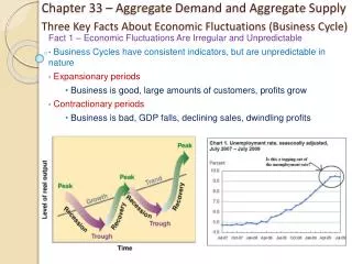
Chapter 33 – Aggregate Demand and Aggregate Supply. Three Key Facts About Economic Fluctuations (Business Cycle). Fact 1 – Economic Fluctuations Are Irregular and Unpredictable Business Cycles have consistent indicators, but are unpredictable in nature Expansionary periods

E N D
Chapter 33 – Aggregate Demand and Aggregate Supply Three Key Facts About Economic Fluctuations (Business Cycle) Fact 1 – Economic Fluctuations Are Irregular and Unpredictable Business Cycles have consistent indicators, but are unpredictable in nature Expansionary periods Business is good, large amounts of customers, profits grow Contractionary periods Business is bad, GDP falls, declining sales, dwindling profits
Three Key Facts About Economic Fluctuations Fact 2 – Most Macroeconomic Quantities Fluctuate Together Real GDP is the most commonly used economic indicator to measure short-run changes in the economy Fall in real GDP, fall in personal income, corporate profits, consumer spending, investment spending, retail sales, home sales, auto sales, etc.
Three Key Facts About Economic Fluctuations Fact 3 – As Output Falls, Unemployment Rises An economy’s output is strongly correlated with utilization of its labor force Real GDP declines, unemployment rises Contraction/Recession, unemployment rises Recession ends, recovery/expansion, unemployment rates fall GDP
Explaining Short-Run Economic Fluctuations • Monetary Neutralitydoes not apply in the short run (6 months, 1 year) • Real and nominal variables are highly intertwined in the short run • “Keep Our Educators Working” bailout of 2009 • Changes in the money supply can temporarily push real GDP away from its long-run trend
Model of aggregate demand & aggregate supply Price Level • Model used to explain short-run fluctuations in economic activity around its long-run trend • Aggregate – a sum, gross amount, of all supply and demand in an economy • Two axes: • Economy’s output of goods and services • Average level of prices (CPI or GDP Deflator) Aggregate supply (AS) Equilibrium price level Aggregate demand (AD) Quantity of Output Equilibrium output
Aggregate Demand Price Level • Aggregate demand curve • Sum of C+I+G+NX (real GDP) at each price level • Downward sloping • Low price levels increase the quantity of goods and services demanded, vice versa Aggregate demand (AD) Quantity of Output CIGNX
Why is the AD Curve Downward Sloping? Price Level • Wealth effect – when prices levels fall consumers feel wealthier, when price levels are high they feel poorer • Interest rate effect – a lower price level reduces interest rates, which stimulates the demand for big ticket consumer goods and investment • Exchange Rate effect – currency depreciates, which makes U.S. exports more competitive internationally, vice versa Aggregate demand (AD) Quantity of Output CIGNX
Why the AD Curve Might Shift? • C - Shifts arising from changes in consumption • Increases in spending – people have more disposable income • Decreases in spending – people become more concerned with saving for retirement • I - Shifts arising from changes in investment • Change in firm investing – tax policy, pessimism about the economy in future, high interest rates • G - Shifts arising from changes in government purchases • Congress increases/decreases spending • NX - Shift arising from changes in net exports • Global recessions would cause a decrease in demand for U.S. products
What Shifts the Aggregate Demand Curve? A C B Price Level C Quantity of Output A C C A A
The Aggregate Supply Curve • AS curve – total quantity of goods and services firms can produce and sell at any given price level • Shape of AS curve depends on time horizon • Short run - Aggregate-supply curve is upward sloping • What shifts the curve? • Temporary changes in Land, Labor, Capital
What Shifts the Aggregate Supply Curve? A C B Price Level A Quantity of Output A C C C C
Aggregate Demand or Supply? AS AS AD AD AD AS AS AS AD AD
AD AS Scenarios Price Level • A significant increase in world oil prices • Government announces a large increase in spending on health and education • Average wage rises way above inflation for the third month running • Exchange rate appreciation knocks export hopes for manufacturing • US productivity levels at their highest level for 10 years • A booming stock market leads to highest rate of retail sales in a century AS AS1 Pe1 Pe AD Quantity of Output Y1 Y
AD AS Scenarios Price Level • A significant increase in world oil prices • Government announces a large increase in spending on health and education • Average wage rises way above inflation for the third month running • Exchange rate appreciation knocks export hopes for manufacturing • US productivity levels at their highest level for 10 years • A booming stock market leads to highest rate of retail sales in a century AS Pe1 Pe AD AD1 Quantity of Output Y Y1
The Aggregate Supply Curve Price Level • In the Long-Run (LRAS) the supply is vertical • Conceptually, the same as the Production Possibilities Curve • An economy’s production of goods and services (real GDP) is based on the factors of production not on price levels • Land, Labor, Capital determine what is possible to produce • LRAS – shows potential output/full employment/natural rate of output • Shows what the economy produces when unemployment is at its natural/normal rate (5-6%) Long-run Aggregate Supply (LRAS) Capital Goods Quantity of Output (GDP) Natural rate of output (GDP)Full Employment 5-6% Consumer Goods
Why the LRAS Curve Might Shift • Changes in Labor • Immigration increase quantity of labor, shift right • Emigration, workers leave for jobs abroad, shift left • Changes in Capital • Increase capital stock (machinery, factories, operating equipment), shift right • Decrease productivity (generational trend to bypass college education), shift left • Changes in Natural Resources • Discovery of oil, shift to right • Cold weather destroys crops, shift to left • Changes in Technological Knowledge • Innovations (computer, internet, handheld devices), shift right • Government policies (environmental concerns, patents, workers safety), shift to left
The Long-Run Equilibrium Long-run aggregate Supply (LRAS) Price Level Short-run aggregate Supply (SRAS) A Equilibrium Price (Ple) Aggregate Demand (AD) Quantity of Output Natural rate of output (Qfe, Y) 5-6% Unemployment • Long-Run-Equilibrium • AD intersects with SRAS and LRAS(point A). • Expected price level has adjusted to equal the actual price level. • Full Employment (natural rate of output), wage Equilibrium
Recessionary and Inflationary Gaps Price Level Price Level LRAS LRAS SRAS SRAS AD AD Q1 (8.2%) 13.4 – T Q1 (2%) 18 – T • Recessionary Gap • Underperforming economy (contraction/recession) • Not at full employment • Unused resources • Falling Prices Quantity of Output(GDP) Quantity of Output(GDP) • Inflationary Gap • Overperforming economy (expansion) • Above full employment • Quickly Rising Prices Qfe (5-6%) GDP – 14 T Qfe (5-6%) GDP – 14 T
Four Step Process For Modeling AS&AD • First, determine whether the event affects AD or AS • Second, determine which way the curve shifts • Third, use AD & AS to compare initial & new equilibrium • Fourth, examine the transition between SRAS and LRAS The Aggregate Demand and Aggregate Supply Model at Long-Run Equilibrium
Effects of a Shift in AD Price Level LRAS • Scenario: The economy is experiencing a recession *Assume long-run equilibrium* • Step 1 – AD or AS affected?AD • Step 2 – Which direction will the curve shift?Left • Step 3 – Plot the new EP (B) • Step 4 – Examine transition between SRAS and LRAS (C) SRAS1 SRAS2 C B 3. . . . Over time, nominal wages come down, price levels decrease(cost of doing business), and the short-run aggregate-supply curve shifts, bringing us back to long-run equilibrium. . . A Ple3 Ple1 Ple2 4. . . . and output returns to its natural rate. • A decrease in • aggregate demand . . . AD2 AD1 Quantity of Output Y2 Y1 2. . . . causes output to fall in the short run, companies lay off workers, unemployment will rise, cut back on production. . .
Effects of a Shift in Demand LRAS Price Level • Scenario: The economy experiences a boom in the stock market, people have more disposable income to spend *Assume long-run equilibrium* • Step 1 – AD or AS affected?AD • Step 2 – Which direction will the curve shift?Right • Step 3 – Plot the new EP (B) • Step 4 – Examine transition between SRAS and LRAS (C) A SRAS1 B C Ple3 Ple1 Ple2 SRAS2 Quantity of Output Y2 Y1 AD2 AD1
Important points about AD • Short run, shifts in AD cause fluctuations in output • Long run, shifts in AD affect overall price level, but not output because we will always return to long run equilibrium • Policymakers can affect AD/AS and reduce the impact of short-run economic fluctuations
Effects of a Shift in AS 3. . . . and the price level to rise (stagflation). . . 2. . . . causes output to fall. . . Price Level LRAS 4. . . . but keeps output at its natural rate. 1. An adverse shift in the short-run AS curve. . . • Scenario: A hurricane hits and reduces the availability of refineries to produce oil *Assume long-run equilibrium* • Step 1 – AD or AS affected?AS • Step 2 – Which direction will the curve shift?Left • Step 3 – Plot the new EP (B) • Step 4 – Examine transition between SRAS and LRAS (C) SRAS2 SRAS1 C A Ple1 Ple3 Ple2 AD1 AD2 B Quantity of Output Y1 Y2 Policymakers affect AD through monetary/fiscal policy. . .
Important points about AS • Short run, shifts in AS can cause stagflation • Long run, shifts in AS affect overall price level, but not output • Policymakers can reduce the impact of economic fluctuations, but risk increasing price levels
Binder Check Chapter 33 • An Introduction to Aggregate Supply and Demand • Short Run AD and AS • Youtube video - (Macro) Episode 24: AD & AS • Youtube video - (Macro) Episode 25: Macroeconomic Viewpoints • Youtube video - (Macro) Episode 26: Macroeconomic Viewpoints • Chapter 33 Mankiw Practice • Free Response • Daily Tens • Notes Chapter 33 • Terms
Extra Credit • How are the LRAS model and the PPC model similar? • Draw a properly labeled graph of each of the above models to show an underperforming (below full employment) economy. • Identify each of the following as being either AS or AD. • Oil refineries • China imports US soybeans • A baseball stadium • A customer buys a hotdog at a baseball game • Each of the following are current event headlines in the news today. List which of the following will most likely to be affected, AD, SRAS, or LRAS. • US drought affects wheat and soybean yields • Despite No Fed Action, Interest Rates For Mortgages Drop To Record Lows • Stock Market Hit Hard By Lack Of QE3 (quantitative easing 3)
Why The Short Run Aggregate-Supply Curve Slopes Upward Price Level Short-run aggregate supply • Key difference in the economy in the short and long run is behavior of AS • Long run, price level does not affect economic output • Short run, price level does affect economic output • Period of a year or two, an increase in price levels raises output • Price levels increase, suppliers want to supply more, vice versa P2 P1 1. A decrease in the price level . . . Quantity of Output Y1 Y2 2. . . . reduces the quantity of goods and services supplied in the short run
Why the AS curve slopes upward in short-run • Sticky-wage theory - nominal wages are slow to adjust to changing economic conditions • Wages are “sticky” in short run • Can affect long-term contracts: workers and firms (up to 3 years) • Nominal wages are based on expected prices • Don’t respond immediately when actual price level is different from what was expected, causing input costs for the firm to increase
Why the AS curve slopes upward in short-run • Sticky-price theory - prices of some goods & services slow to adjust to changing economic conditions • Menu costs, firms’ costs of adjusting prices
Why the AS curve slopes upward in short-run • Misperceptions theory - changes in the overall price level can temporarily mislead suppliers about changes in individual markets • Suppliers respond to changes in level of prices change quantity supplied of goods and services