Download
1 / 1
10 likes | 151 Views
This study presents an innovative approach for improving error covariance estimation in the ARM variational analysis framework, specifically targeting atmospheric state variables. By utilizing an AR(1) model, we examine and characterize error structures that enhance the accuracy of cost function minimization for multivariable analyses, such as the TWP-ICE experiment. The methodology allows for effective inversion of the covariance matrix, capturing essential correlations among different levels, which ultimately improves the quality of data analysis. Ongoing testing and implementation of this numerical algorithm aim to refine the variational analysis further.

E N D
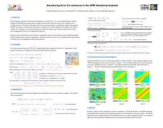
It can be shown that from an AR(1) model that: where are similarly defined. are similarly defined. are calculated from the data. or where where and so on. Introducing Error Co-variances in the ARM Variational Analysis Minghua Zhang (Stony Brook University/SUNY) and Shaocheng Xie (Lawrence Livermore National Laboratory) ITPA 1. Introduction Any optimization algorithm involves the minimization of a cost function. For multi-variable analysis, such as analysis of ARM data with several stations, many levels and time steps, the cost function contains a error covariance matrix. Elements of the matrix determines how observations are weighted to produce the analysis. In NWP community, it is well known that the error covariance has a major impact on the quality of the optimal analysis. For example, if several measurements are highly correlated, each individual data entry should be given small weight relative to an independent data entry. Because of the complexities to derive the error covariance matrix from actual data, the current ARM variational analysis assumes that errors are independent. Since most of the errors are due to sampling rather than random instrument error, this assumption needs to be improved. To obtain an AR(1) model is used such that: Covariance between two levels for other variables can be similarly calculated. It can be also shown that: This is a symmetric polynomial matrix that can be inverted using the Cholesky decomposition. When the correlation length scale is short, it is a narrow diagonal matrix. can be similarly obtained. The analysis is then calculated from: 2. The Problem For a field experiment such as TWP-ICE, the atmospheric state variables of winds (u,v), temperature () and specific humidity (q) at S stations, K levels, and N time steps are written as with constraints: The merit of the above matrix structure is that it yields an explicit solution from the cost function term in the E-L equation. 4. Error Structures and Correlation Matrices Analysis increments or errors in observations relative to the first iteration of the variational analysis for the TWP-ICE temperature and u wind are shown in Figure 1. The correlation matrices in the vertical direction for the two variables are shown in Figure 2. The matrices derived from the AR1 model are shown in Figure 3. The AR(1) model captures the general features of the correlations. Similarly and With truth & observations as: and We write errors: and Maximum likelihood or minimum variance leads to cost function: is populated by covariance among all stations/levels/variables/ time steps. The dimension of this matrix is In TWP-ICE, this is (4X45X6X201)^2 = 2170802 The minimization of I is subject to the five constraints of column integrated conservations at each time step: Not only this matrix is too large to invert, but also the covariance cannot be easily obtained from data. 3. A New Method Since the constraints are vertically integrated, we first assume errors to be vertically correlated. This reduces the cost function to: Where Figure 2 Figure 3 Figure 1 5. Summary An AR(1) model is used to characterize the error covariance in the vertical direction in the ARM variational analysis that allows inversion of the covariance matrix for the minimization of the cost function. The model captures the de-correlation lengths and the different matrix structures for different variables. The numerical algorithm is being tested and implemented into the variational analysis of TWP-ICE data. These matrices are KXK in dimension.