Download
1 / 74
760 likes | 1.27k Views
INTEGRALS. 5.3 The Fundamental Theorem of Calculus. In this section, we will learn about: The Fundamental Theorem of Calculus and its significance. FUNDAMENTAL THEOREM OF CALCULUS. The Fundamental Theorem of Calculus (FTC) is appropriately named.

E N D
INTEGRALS 5.3The Fundamental Theorem of Calculus • In this section, we will learn about: • The Fundamental Theorem of Calculus • and its significance.
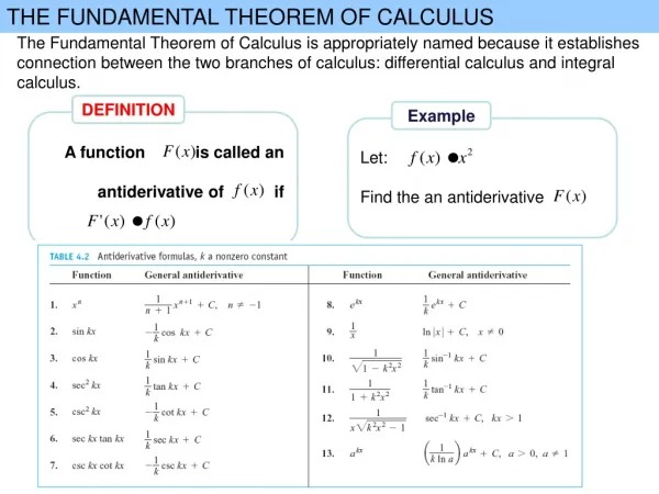
FUNDAMENTAL THEOREM OF CALCULUS • The Fundamental Theorem of Calculus (FTC) is appropriately named. • It establishes a connection between the two branches of calculus—differential calculus and integral calculus.
FTC • Differential calculus arose from the tangent problem. • Integral calculus arose from a seemingly unrelated problem—the area problem.
FTC • Newton’s mentor at Cambridge, Isaac Barrow (1630–1677), discovered that these two problems are actually closely related. • In fact, he realized that differentiation and integration are inverse processes.
FTC • The FTC gives the precise inverse relationship between the derivative and the integral.
FTC • It was Newton and Leibniz who exploited this relationship and used it to develop calculus into a systematic mathematical method. • In particular, they saw that the FTC enabled them to compute areas and integrals very easily without having to compute them as limits of sums—as we did in Sections 5.1 and 5.2
FTC Equation 1 • The first part of the FTC deals with functions defined by an equation of the form • where f is a continuous function on [a, b] and x varies between a and b.
FTC • Observe that g depends only on x, which appears as the variable upper limit in the integral. • If x is a fixed number, then the integral is a definite number. • If we then let x vary, the number also varies and defines a function of x denoted by g(x).
FTC • If f happens to be a positive function, then g(x) can be interpreted as the area under the graph of f from a to x, where x can vary from a to b. • Think of g as the ‘area so far’ function, as seen here.
FTC Example 1 • If f is the function whose graph is shown and , find the values of: g(0), g(1), g(2), g(3), g(4), and g(5). • Then, sketch a rough graph of g.
FTC Example 1 • First, we notice that:
FTC Example 1 • From the figure, we see that g(1) • is the area of a triangle:
FTC Example 1 • To find g(2), we add to g(1) the area of a rectangle:
FTC Example 1 • We estimate that the area under f from 2 to 3 is about 1.3. • So,
FTC Example 1 • For t > 3, f(t) is negative. • So, we start subtracting areas, as follows.
FTC Example 1 • Thus,
FTC Example 1 • We use these values to sketch the graph of g. • Notice that, because f(t) is positive for t < 3, we keep adding area for t < 3. • So, g is increasing up to x = 3, where it attains a maximum value. • For x > 3, g decreases because f(t) is negative.
FTC • If we take f(t) = t and a = 0, then, using Exercise 27 in Section 5.2, we have:
FTC • Notice that g’(x) = x, that is, g’ = f. • In other words, if g is defined as the integral of fby Equation 1, g turns out to be an antiderivative of f—atleastin this case.
FTC • If we sketch the derivative of the function g,as in the first figure, by estimating slopes of tangents, we get a graph like that of f in the second figure. • So, we suspect that g’ = fin Example 1 too.
FTC • To see why this might be generally true, we consider a continuous function f with f (x) ≥ 0. • Then, can be interpreted as the area under the graph of f from a to x.
FTC • To compute g’(x) from the definition of derivative, we first observe that, for h > 0, g(x + h) – g(x) is obtained by subtracting areas. • It is the area under the graph of f from x to x + h (the gold area).
FTC • For small h, we see that this area is approximately equal to the area of the rectangle with height f(x) and width h: • So,
FTC • Intuitively, we therefore expect that: • The fact that this is true, even when f is not necessarily positive, is the first part of the FTC (FTC1).
Fundamental Theorem of Calculus Version 1 • If f is continuous on [a, b], then the function g defined by • is continuous on [a, b] and differentiable on (a, b), and g’(x) = f(x).
FTC1 • In words, the FTC1 says that the derivative of a definite integral with respect to its upper limit is the integrand evaluated at the upper limit.
FTC1 • Using Leibniz notation for derivatives, we can write the FTC1 as • when f is continuous. • Roughly speaking, Equation 5 says that, if we first integrate f and then differentiate the result, we get back to the original function f.
FTC1 Example 2 • Find the derivative of the function • As is continuous, the FTC1 gives:
FTC1 • A formula of the form may seem like a strange way of defining a function. • However, books on physics, chemistry, and statistics are full of such functions.
FRESNEL FUNCTION Example 3 • For instance, consider the Fresnel function • It is named after the French physicist Augustin Fresnel (1788–1827), famous for his works in optics. • It first appeared in Fresnel’s theory of the diffraction of light waves. • More recently, it has been applied to the design of highways.
FRESNEL FUNCTION Example 3 • The FTC1 tells us how to differentiate the Fresnel function: • This means that we can apply all the methods of differential calculus to analyze S.
FRESNEL FUNCTION Example 3 • The figure shows the graphs of f (x) = sin(πx2/2) and the Fresnel function • A computer was used to graph S by computing the value of this integral for many values of x.
FRESNEL FUNCTION Example 3 • It does indeed look as if S(x) is the area under the graph of f from 0 to x (until x ≈ 1.4, when S(x) becomes a difference of areas).
FRESNEL FUNCTION Example 3 • The other figure shows a larger part of the graph of S.
FRESNEL FUNCTION Example 3 • If we now start with the graph of S here and think about what its derivative should look like, it seems reasonable that S’(x) = f(x). • For instance, S is increasing when f(x) > 0 and decreasing when f(x) < 0.
FRESNEL FUNCTION Example 3 • So, this gives a visual confirmation of the FTC1.
FTC1 Example 4 • Find • Here, we have to be careful to use the Chain Rule in conjunction with the FTC1.
FTC1 Example 4 • Let u = x4.Then,
FTC1 • In Section 5.2, we computed integrals from the definition as a limit of Riemann sums and saw that this procedure is sometimes long and difficult. • The second part of the FTC (FTC2), which follows easily from the first part, provides us with a much simpler method for the evaluation of integrals.
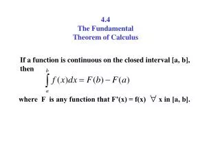
Fundamental Theorem of Calculus Version 2 • If f is continuous on [a, b], then • where F is any antiderivative of f, that is, a function such that F ’ = f.
FTC2 Proof • Let • We know from the FTC1 that g’(x) = f(x), that is, g is an antiderivative of f.
FTC2 Proof—Equation 6 • If F is any other antiderivative of f on [a, b], then we know from Corollary 7 in Section 4.2 that F and g differ by a constant • F(x) = g(x) + C • for a < x < b.
FTC2 Proof • However, both F and g are continuous on [a, b]. • Thus, by taking limits of both sides of Equation 6 (as x→ a+and x→ b- ), we see it also holds when x = a and x = b.
FTC2 Proof • If we put x = a in the formula for g(x), we get:
FTC2 Proof • So, using Equation 6 with x = b and x = a, we have:
FTC2 • The FTC2 states that, if we know an antiderivative F of f, then we can evaluate simply by subtracting the values of F at the endpoints of the interval [a, b].
FTC2 • It is very surprising that , which was defined by a complicated procedure involving all the values of f(x) for a≤ x ≤ b, can be found by knowing the values of F(x) at only two points, a and b.
FTC2 • At first glance, the theorem may be surprising. • However, it becomes plausible if we interpret it in physical terms.
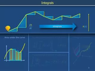
FTC2 • If v(t) is the velocity of an object and s(t) is its position at time t, then v(t) = s’(t). • So, s is an antiderivative of v.
FTC2 • In Section 5.1, we considered an object that always moves in the positive direction. • Then, we guessed that the area under the velocity curve equals the distance traveled. • In symbols, • That is exactly what the FTC2 says in this context.