Download
1 / 28
280 likes | 334 Views
Explore concepts of data interpolation, image resizing methods, general interpolation functions, enlargement by spatial filtering, scaling smaller images, and techniques for image rotation and anamorphosis. Understand the importance of interpolating surrounding values to enhance image quality.

E N D
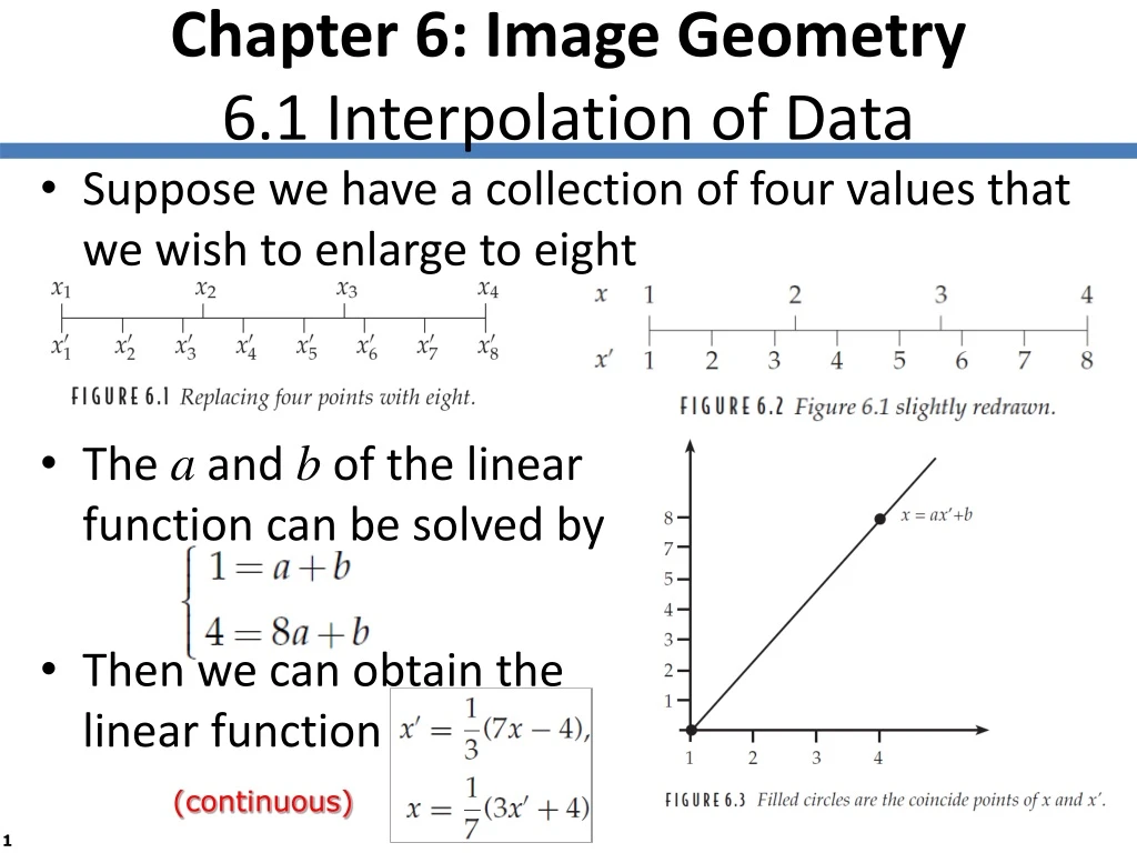
Chapter 6: Image Geometry6.1 Interpolation of Data • Suppose we have a collection of four values that we wish to enlarge to eight • The a and b of the linear function can be solved by • Then we can obtain the linear function (continuous)
6.1 Interpolation of Data • In digital (discrete), none of the points coincide exactly with an original xj, except for the first and last • We have to estimate function values based on the known values of nearby f (xj) • Such estimation of function values based on surrounding values is • called interpolation • Nearest-neighbor interpolation
FIGURE 6.5 • Linear interpolation (Equation 6.1)
6.2 Image Interpolation • Using the formula given by Equation 6.1 bilinear interpolation
6.2 Image Interpolation • Function imresize • Where A is an image of any type, k is a scaling factor, and ’method’ is either ’nearest’ or ’bilinear’, etc.
6.3 General Interpolation • Generalized interpolation function: • R0(u) Nearest-neighbor interpolation (Equation 6.2)
6.3 General Interpolation • R1(u) Linear interpolation • Cubic interpolation
6.4 Enlargement by Spatial Filtering • If we merely wish to enlarge an image by a power of two, there is a quick and dirty method that uses linear filtering • e.g. • zero-interleaved
FIGURE 6.17 • This can be implemented with a simple function
6.4 Enlargement by Spatial Filtering • We can now replace the zeros by applying a spatial filter to this matrix nearest-neighbor bilinear bicubic
6.5 Scaling Smaller • Making an image smaller is also called image minimization • Subsampling • e.g.
6.6 Rotation • In Figure 6.21, the filled circles indicate the original position, and the open circles point their positions after rotation • We must ensure that even after rotation, the points remain in that grid • To do this we consider a rectangle that includes the rotated image, as shown in Figure 6.22
6.6 Rotation • The gray value at (x”, y”) can be found by interpolation, using surrounding gray values. This value is then the gray value for the pixel at (x’, y’) in the • rotated image


