Download
1 / 41
410 likes | 569 Views
The Acceleration of the Universe. Ruth A. Daly. Review of Data Indicating that the Universe is Accelerating. 1). Observations of the Cosmic Microwave Background Radiation → Space curvature = 0

E N D
The Acceleration of the Universe Ruth A. Daly
Review of Data Indicating that the Universe is Accelerating 1). Observations of the Cosmic Microwave Background Radiation → Space curvature = 0 Numerous types of local measurements → Ωm ~ 0.3 (Clusters of Galaxies, LSS, Flows,….Age Problem ….) + Flat Universe → Dark Energy (CMB + Detailed Modeling → Dark Energy + an Accelerating Universe) 2). Type Ia Supernovae → Universe is Accelerating Radio Galaxies → Universe is Accelerating
CMBAngular Power Spectrum Observations of the Cosmic Microwave Background → Space curvature = 0
157 Type Ia SN: Constraints in a Λ model (Riess et al. 2004)
Radio Galaxy Constraints in a quintessence model (Daly & Guerra 2002).
54 SN in a k=0 Quintessence model, w=P/ρ 54 SN in a k=0 quintessence model (from DG02)
20 RG + 54 SN in a Quintessence Model Results with 20 RG + 54 SN (from DG02)
The CMB + Any One of Many Types of Local Measurements (→ Ωm ~ 0.3) → Dark Energy and an Accelerating Universe Type Ia Supernovae alone → An Accelerating Universe FRIIb Radio Galaxies alone → An Accelerating Universe
Recent Results from DD03 & DD04The SN and RG methods → a set of luminosity or coordinate distances y(z)= Hoaor (z)
For k=0, (aor) = ∫ dt/a(t) = ∫ (á/a)-1 dz 1). Method 1: select GR & fE(z,w); use data to obtain the best fit values of the model. Einstein Equations (for k=0): (á/a)2=(8πG/3)∑ρi =Ho2[Ωom(1+z)3 + fE(z,w)] where ρE(z) = ρ0c fE(z,w) and w = PE /ρE ä/a= -(4πG/3)∑(ρi+3Pi) = -(4πG/3)[ρm+ρE+3PE] 2). Method 2: Differentiate the data aor(z) or y(z) + solve directly for q(z) = - äa/(á)2, E(z) = (á/a); can also obtain PE(z), ρE(z), and w(z) [DD03,04] q(z) and E(z) only depend upon the FRW metric!
Rather than assuming GR and integrating a model for fE(z,w) to obtain the best fit model parameters, we take y(z) to each source, do a robust numerical differentiation, solve for dy/dz and d2y/dz2→ obtainthe dimensionless expansion and acceleration rates: E(z) = (á/a)/Ho = (dy/dz)-1 q(z)=-äa/(á)2=-[1+(1+z)(dy/dz)-1(d2y/dz2)] Only assumes FRW (Valid for any homogeneous, isotropic space-time)!→ Independent of GR & Models
Derivation dτ2=dt2 – a2(t)[dr2/(1-kr2)+r2dθ2+r2sin2θ dφ2] for a light ray from source, dt=a(t)dr when k=0; dz/dt = -ao-1 (1+z)(dr/dz) since (1+z) = ao/a(t). Differentiating this, ά= -ao (1+z)-2 (dz/dt) = (1+z)-1(dr/dz)-1, or, with y = H0(a0r) H(z) ≡ (ά/a) = (d(aor)/dz)-1 = Ho (dy/dz)-1. → E(z) ≡ H(z)/Ho = (dy/dz)-1(Weinberg 1972) Differentiating ά,→ ä=-(1+z)-2 (dz/dt) (dr/dz)-1 [1+(1+z)(dr/dz)-1 (d2r/dz2)] or q(z)≡-(äa)/ά2=-[1+(1+z)(dy/dz)-1 d2y/dz2] (DD03) So, E(z) and q(z) can be obtained independent of GR & of specific models for the “dark energy!”
The Methodology y(z) Fit a parabola in a sliding window of ∆z around some z0 From the local fit coefficients, get y(z0), dy/dz and d2y/dz2 and their errors z0 z This is equivalent to a local Taylor expansion for y(z); a parabola is a minimum assumption local model for y(z). For noisy/sparse data, need a large ∆z: poor redshift resolution, but can determine trends …
Testing the Methodology Using Simulated (Pseudo-SNAP) Data From DD03; Assumes m = 0.3, = 0.7, and z = 0.4
Initial results for the evolution of the expansion rate E(z) and the acceleration parameter q(z), obtained using 20 RG and 78 SNFound zT ≈ 0.45from DD03
Good agreement between RG and SN E(z) = (dy/dz)-1 From DD03; using 20 RG and 78 SN
New Results: Coordinate Distances y(z)157 Gold SN Sample + 20 RG
Comparison of SN and RG Distances In what follows, SN-only sample gives essentially the same results; RGs help tighten the error bars at the high-z end.
Valid for any theory of gravity, and any type of “DE”; only assumes k=0 and FRW metric Evolution of the Cosmic Acceleration - Transition redshift: zT ~ 0.4 q0= -.35 ±.15
Evolution of the Cosmic Acceleration Valid for any theory of gravity, and any type of “DE”; only assumes k=0 and FRW metric - Transition redshift: zT ~ 0.4 q0= -.35 ±.15
Can solve for the pressure PE, Energy Density fE, and equation of state w of the Dark Energy if a theory of gravity is assumed. Einstein Equations (for k=0): ä/a= - (4πG/3) [ρm + ρE + 3 PE] (á/a)2 = (8πG/3) [ρm + ρE] → PE = [E2(z)/3] [2 q(z) -1] or pE(z)=-(dy/dz)-2[1+(2/3)(1+z)(dy/dz)-1(d2y/dz2)], where pE(z)≡PE/ρoc With FRW + GR, we have PE(z)!
Pressure of the Dark Energy (Assumes GR) For models, p=- → direct measure of Λ We measure p0 = -0.60 ± 0.15 Since ρ0E= p0/w0, Ω0E = 0.60 ±0.15for w0 = -1
The Energy Density fE and equation of state w of the Dark Energy can be obtained if we assume a theory of Gravity and adopt a value of Ωm: Einstein Equations (for k=0): (á/a)2 = (8πG/3) [ρm + ρE] ä/a= - (4πG/3) [ρm + ρE + 3 PE] → fE(z) ≡ ρE(z)/ρoc = (dy/dz)-2 – Ωm(1+z)3 w(z) = -[1+(2/3)(1+z)(dy/dz)-1(d2y/dz2)/ [1-(dy/dz)2 Ωm(1+z)3], where w(z) = pE(z)/fE(z) = eq. of state
Relative Energy Density of the Dark Energy f0=0.62 ± 0.04
Evolution of the EOS Parameter w(z) We measure w0 = -0.9 0.1 Consistent with models, but possible evolution
Summary The Acceleration of the Universe is indicated by: CBM Obs. + Local Obs. → (k=0 + Ωm ~ 0.3); + Supernovae Type Ia (and Radio Galaxy) Obs. Though these determinations are model dependent, very similar results are obtained using different models (e.g. Λ, quintessence, ….); assumes GR. It is possible to use SN and RG observations to determine E(z), q(z), P(z), f(z), w(z), etc. in a model-independent fashion.
Assuming Only: Flatness + FRW → q(z) and E(z). Find that the universe is accelerating today, and was decelerating in the recent past (R.D. + Djorgovski 2003,2004). • + GR can solve for p(z) • For models, = -p → direct measure of Λ (independent of other methods) • + Ωom → ρE(z) and w(z) • Transition found by DD03 from accelerating to decelerating universe at zT ~ 0.4 is confirmed by DD04; Agrees with Riess et al. (2004) • Perhaps a hint that w is evolving with redshift • The current data provide some useful constraints for theoretical models; generally consistent with “concordance cosmology” (m ≈ 0.3, ≈ 0.7)
Evolution of the Cosmic Acceleration Valid for any theory of gravity, and any type of “DE”; only assumes k=0 and FRW metric - Transition redshift: zT ~ 0.4 q0= -.35 ±.15
Pressure of the Dark Energy (Assumes GR) For models, p=- → direct measure of Λ We measure p0 = -0.60 ± 0.15 Since ρ0E= p0/w0, Ω0E = 0.60 ±0.15for w0 = -1