Download
1 / 15
150 likes | 276 Views
2011 ADSA-ASAS Joint Annual Meeting New Orleans, LA, July 10-14. A recursive method of approximation of the inverse of genomic relationship matrix. P. Faux * ,1 , I. Misztal 2 , N. Gengler 1,3 1 University of Liège, Gembloux Agro-Bio Tech, Belgium

E N D
2011 ADSA-ASAS Joint Annual Meeting New Orleans, LA, July 10-14 A recursive method of approximation of the inverse of genomic relationship matrix P. Faux *,1, I. Misztal2, N. Gengler 1,3 1University of Liège, Gembloux Agro-Bio Tech, Belgium 2University of Georgia, Animal and Dairy Science, Athens GA 3National Fund for Scientific Research, Brussels, Belgium * Supported by the National Research Fund, Luxembourg (FNR)
Introduction • Inverse of genomicrelationship matrix (G) usefulin differentgenomicevaluations: single-step, multiple-steps • Inversion becomes time-consumingwhennumber of genotypedanimals>50,000 • A good approximation of Ginverse willbecomeuseful 2011 ADSA-ASAS Joint Annual Meeting, New Orleans, July 10-14
Methods: Approximated inverse of G • Decompositionof A-1: A-1=(T-1)’ . D-1 . T-1 • We assume the following model for G-1: G-1=(T*)’ . (D-1)* . T* + E Or, (G-1)*=(T*)’ . (D-1)* . T* • 2 approximations have to bedone: T* and (D-1)* 2011 ADSA-ASAS Joint Annual Meeting, New Orleans, July 10-14
Methods: Case of A-1 • Animal a, of sire s and dam d: A T-1 A x b = - 2011 ADSA-ASAS Joint Annual Meeting, New Orleans, July 10-14
Methods: Case of G-1 G T* A x b = - 2011 ADSA-ASAS Joint Annual Meeting, New Orleans, July 10-14
Methods: Case of G-1 G T* A x b = - 2011 ADSA-ASAS Joint Annual Meeting, New Orleans, July 10-14
Methods: Approximation of D-1 (G-1)*=(T*)’ . (D-1)* . T* D = T* . G. (T*)’ • D close to diagonal 2 options: • Invert only diagonal elements (D-1)* is a diagonal matrix • Apply the same rules as for approximation of G-1 but for D-1 (D-1)* is a sparse matrix (D-1)*=(T2*)’ . (D2-1)* . T2* 2011 ADSA-ASAS Joint Annual Meeting, New Orleans, July 10-14
Methods: Recursive approximation • Same recursion may be repeated n times on the “remaining D” (G-1)*n=(T*1)’ . ... . (T*n)’ . (Dn-1)* . T*n . ... . T*1 • At each round, new threshold p • 2 computational bottle-necks are shown in this equation • Algorithm may be implemented in different ways 2011 ADSA-ASAS Joint Annual Meeting, New Orleans, July 10-14
Examples: Material • Dairy bulls data set: • 1,718 genotyped bulls • 38,416 SNP • Single-step genomic evaluations on Final Score, each evaluation uses a different (G-1)* • Construction of G: • G=ZZ’/d • Both diagonals and off-diagonals of G centered on A22 2011 ADSA-ASAS Joint Annual Meeting, New Orleans, July 10-14
Examples: Quality of approximation • Mean square difference (MSD) between G-1 and (G-1)* • MSD between G-1 and A22-1: 81.49*10-4 2011 ADSA-ASAS Joint Annual Meeting, New Orleans, July 10-14
Examples: Incidence on evaluation • Correlations r between EBV for genotyped animals • r between G-1 and A22-1: 0.76 2011 ADSA-ASAS Joint Annual Meeting, New Orleans, July 10-14
Examples: Sparsity • Percentage of zeros in lower off-diagonal part of Tf 2011 ADSA-ASAS Joint Annual Meeting, New Orleans, July 10-14
Examples: Othersresults • Use of this algorithm to compute (A22-1)* • Closeness with A22-1: from 2*10-4 to 3*10-5 • No incidence on evaluations after 3 rounds • 93% of 0 after 1 round, ... up to ~80% 2011 ADSA-ASAS Joint Annual Meeting, New Orleans, July 10-14
Discussion • Consumption of time • Savings on both bottle-necks • Might be interesting in some cases • Construction of consistent relationships and covariances 2011 ADSA-ASAS Joint Annual Meeting, New Orleans, July 10-14
Acknowledgements • Animal and Dairy Science (ADS) Department of University of Georgia (UGA), for hosting and advising (Mrs H. Wang, Dr S. Tsuruta, Dr I. Aguilar) • Animal Breeding and GeneticsGroup of Animal Science Unit of Gembloux Agro-Bio Tech of University of Liège (ULg –Gx ABT) • Holstein Association USA Inc. for providing data 2011 ADSA-ASAS Joint Annual Meeting, New Orleans, July 10-14