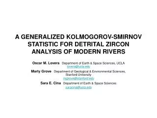
A GENERALIZED KOLMOGOROV-SMIRNOV STATISTIC FOR DETRITAL ZIRCON ANALYSIS OF MODERN RIVERS

1. A GENERALIZED KOLMOGOROV-SMIRNOV STATISTIC FOR DETRITAL ZIRCON ANALYSIS OF MODERN RIVERS Oscar M. LoveraDepartment of Earth & Space Sciences, UCLA lovera@ucla.edu Marty GroveDepartment of Geological & Environmental Sciences, Stanford University mjgrove@stanford.edu Sara E. CinaDepartment of Earth & Space Sciences saracina@ucla.edu

3. Example of Input Files • Sample data are input as two columns (Age(Ma), 1s(Ma)) files (see example, no head labels). Sample filename length must be at least 2 character and less than 10. Because output filenames are form with the two first characters of each catchment sample, it is preferable that the catchment names do not agree in the 1st two characters of their names. • To calculate the relative erosion rates matrix, a predicted relative catchment contribution vector must be input. It is read from a simple three column file “Predicted.in” (see example), with the predicted relative catchment contributions separate by space or tabs. Be sure that the predicted catchment contributions are given from left to right in the same order that catchment sample filenames were input in the 2nd input screen. • NOTE: Selecting option “a” in the 1st input screen calculates “all” matrices, including relative erosion estimates. If an “Predicted.in” input file is not provided, a “dummy” predicted “uniform” relative contributions (1/3,1/3,1/3) would be used and the resulting erosion probability matrix will be identical to the relative contribution probability matrix. Sample input file X0 Age(Ma) ±s ----------- 336.8 18.2 356.7 16.2 415.8 16.9 430.8 25.0 432.0 24.3 446.2 5.6 448.4 7.1 455.6 7.9 466.7 24.2 485.8 19.9 490.6 13.6 514.2 7.0 515.4 17.9 515.5 17.4 515.6 15.5 519.5 21.4 528.6 34.3 529.6 28.3 551.5 5.9 557.3 4.0 … …. Predicted.in File X1 X2 X3 0.43 0.37 0.20

4. RUNNING THE PROGRAM SELECT THE ROUTINE(S) YOU WANT TO RUN (a) - RUN ALL THE ROUTINES AT ONCE (1) - CALCULATE PDF, CPDF CURVES AND STATISTIC AND CORRELATION VALUES (2) - CALCULATE D MATRIX FOR TERNARY PLOTS (3) - CALCULATE THE PROBABILITY MATRIX (4) - CALCULATE THE EROSION MATRIX (5) - CALCULATE TERNARY CONTOURS (PROB OR EROSION) ENTER SELECTION? (a,1,2,3,4 o 5) a

5. 2nd input screen if 1st selection is ( a,1 or 2) Enter name of Main sample distribution X0 ENTER NAME OF CATCHMENT SAMPLE (STOP to end reading) X1 ENTER NAME OF CATCHMENT SAMPLE (STOP to end reading) X2 ENTER NAME OF CATCHMENT SAMPLE (STOP to end reading) X3 ENTER NAME OF CATCHMENT SAMPLE (STOP to end reading) stop total % sigma average= 3.535128 GENKS DONE

6. 2nd Selection screen if 1st selection is ( 3,4 or 5) ENTER TYPE OF MODEL YOU WANT TO CALCULATE: (1) - INDEPENDENT (2) - IDENTICAL (3) - BOTH 1 GENKS DONE DMATX DONE …. 3rd Selection screen if 1st selection is (5) (1) - CALCULATE CONTOURS OF PROB MATRIX (2) - CALCULATE CONTOURS OF EROSION MATRIX (3) - CALCULATE BOTH CONTOURS (PROB & EROSION) 1 GENKS DONE DMATX DONE PROB_DCRIT_MTX DONE EROSION DONE

7. OUPUT FILES • GenKS.DAT– KS Statistic and Correlation calculations between the Main Trunk sample and the catchment samples (PROB values are not corrected by shifting due to incorporation of experimental error). Note: More than three catchments can be input to calculate KS statistic and Correlation values, but ternary matrices will only be calculated from the first three input catchments. • Name.txt– Age vs. PDF and CPDF values. Column 1 = Age(Ma), Column 2 = PDF and Column 3 = CPDF. Plot them using any X-Y Graph application. • Matrixname_param.dat– Information of the sample and screen input values. Other calculated values like Max. D and Prob., avg. sigma, etc., are also output here. • Matrixname_opt_dist.dat – Age vs. PDF and CPDF values for the optimum Mixture (Max. Probability). (Matrixname = first 2 characters of catchment sample names; i.e. X1_X2_X3). • Matrixname_matx.dat– Matrix of the Max. D values computed between the Mixture and the Main Trunk CPDFs curves. Catchment contributions fi are varying from 0 to 1 at 0.001 intervals (Grid=1000x1000). • Matrixname_prob??.dat – Matrices of the Probability values (id=identical, in=independent populations) • Matrixname_er??.dat – Matrices of the Erosion contributions (id or in) • Matrixname_??_cont.dat – ternary contours calculated from the PROB or erosion matrices. Contours are calculated between 0.05 and the max. probability value of the matrix at 0.05 intervals, plus the contours at the 0.01, 0.001 and 0.0001 values.

8. GenKS.dat File Name.txt File Matrixname_opt_dist.txt File Three column file (X,Y1,Y2) without head labels. Ages between 0 and 4.Ga at 2-12Ga intervals. Avg. % sigma uncertainty quote at the bottom. Optimum Mixture with Max. Prob. Two column file (X,Y1,Y2) without head labels. Ages same as Name.txt.

9. Example of Matrixname_param.dat Total Average % sigma = 3.535128 D-MATRIX SUBROUTINE X N= 201 (Main Trunk Sample) X1 N= 89 X2 N= 98 X3 N= 178 D %S1 %S2 %S3 0.0364 33.7000 35.3000 31.0000 CONTOUR SUBROUTINE Pmax contr: 33.70000 35.30000 31.00000 Plow= 5.0000001E-02 Pmax= 0.4421005 N= 8 5.0000001E-02 0.1000000 0.1500000 0.2000000 0.2500000 0.3000000 0.3500000 0.4000000 ………. average % sigma for all the sample data (X,X1,X2,X3) Size of sample distributions (S1,S2,S3) relative contributions of the mixture with the least max. different (D). Relative contributions of the Mixture with the max. PROB (Pmax). PROB values of the Contours calculated between 0.05 and Pmax.

10. f1/f20.000 0.001 0.002 0.003 0.004 0.005 0.006 0.007 0.000 0.5808 0.58005 0.5793 0.57854 0.57779 0.57704 0.57629 0.57554 0.001 0.57996 0.5792 0.57845 0.5777 0.57695 0.5762 0.57545 0.5747 0.002 0.57911 0.57836 0.57761 0.57686 0.57611 0.57536 0.57461 0.57386 0.003 0.57827 0.57752 0.57677 0.57602 0.57527 0.57452 0.57376 0.57301 0.004 0.57743 0.57668 0.57593 0.57517 0.57442 0.57367 0.57292 0.57217 0.005 0.57659 0.57583 0.57508 0.57433 0.57358 0.57283 0.57208 0.57133 0.006 0.57574 0.57499 0.57424 0.57349 0.57274 0.57199 0.57124 0.57049 0.007 0.5749 0.57415 0.5734 0.57265 0.5719 0.57115 0.57039 0.56964 Example of Matrix File Note: These are triangular matrices. Bottom right triangle values are set to -1. We use them only to calculate ternary contours, but they can be use to plot contours on any 2D graph application.

11. Row # f1f2f3(1) f3(0.05) f3(0.10) f4(0.15) 1 0.5761 0 0.4239 -1 -1 2 0.576 1.27E-4 0.42387 -1 -1 3 0.57527 1E-3 0.42373 -1 -1 4 0.575 0.00133 0.42367 -1 -1 5 0.57444 0.002 0.42356 -1 -1 ... ... ... ... … … 2811 0.035 0.85223 0.11277 -1 -1 2812 0.03517 0.852 0.11283 -1 -1 2813 0.10199 0.736 -1 0.16201 -1 2814 0.102 0.73601 -1 0.16199 -1 2815 0.10201 0.736 -1 0.16199 -1 2816 0.102 0.73596 -1 0.16204 -1 ... ... ... ... ... … 5118 0.10395 0.731 -1 0.16505 -1 5119 0.10353 0.732 -1 0.16447 -1 5120 0.15374 0.651 -1 -1 0.19526 5121 0.154 0.65138 -1 -1 0.19462 5122 0.15424 0.651 -1 -1 0.19476 ... ... ... ... ... … Example of Contour Files Note: Output file is taylor to plot ternary contour using the Origin Graph application. First to columns (f1,f2) are label as X,Y. Columns from 3rd and up (f3) must be designed as Z.

12. Files used: X0.txt, X1.txt, X2.txt, X3.txt and X1_X2_X3_opt_dist.dat

13. RELATIVE CATCHMENT CONTRIBUTIONS PROBABILITY CONTOURS Files used: X1_X2_X3_pmatxin.dat and X1_X2_X3_pmatxid.dat. Note that not all calculated contours were plot.

14. RELATIVE EROSION RATE CONTOURS

15. Glossary Dcrit: Critical D value (i.e. P(Dcrit)=0.05) PDF: Probability Density Function (Gaussian Kernel Probability). CPDF: Cumulative Probability Density Function (Integral of the Gaussian Kernel Probability). CDF: Cumulative Distribution Function CC: Cross-correlation values between two Probability Density Functions (PDF)