Three classic HMM problems

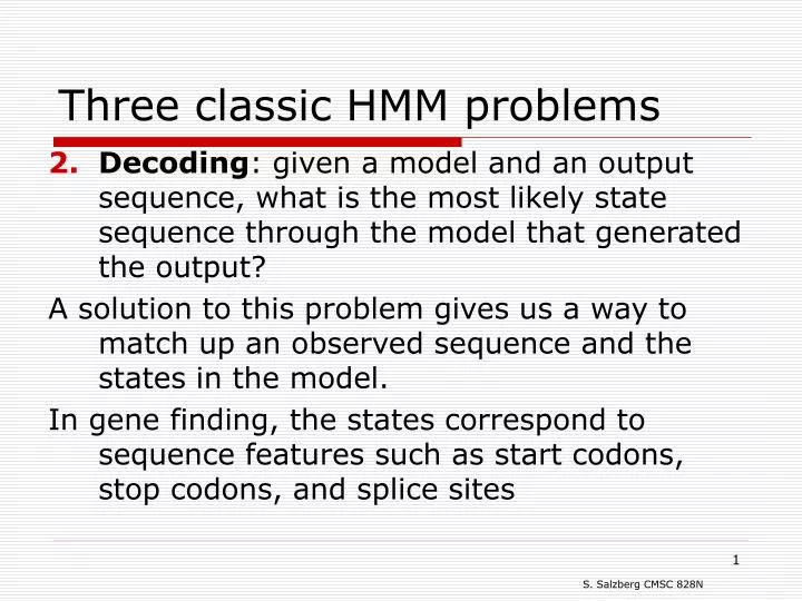
1. Three classic HMM problems • Decoding: given a model and an output sequence, what is the most likely state sequence through the model that generated the output? A solution to this problem gives us a way to match up an observed sequence and the states in the model. In gene finding, the states correspond to sequence features such as start codons, stop codons, and splice sites

2. Three classic HMM problems • Learning: given a model and a set of observed sequences, how do we set the model’s parameters so that it has a high probability of generating those sequences? This is perhaps the most important, and most difficult problem. A solution to this problem allows us to determine all the probabilities in an HMMs by using an ensemble of training data

3. Viterbi algorithm Where Vi(t) is the probability that the HMM is in state i after generating the sequence y1,y2,…,yt, following the most probable path in the HMM

4. Our sample HMM Let S1 be initial state, S2 be final state

5. Time t=1 t=2 t=3 t=0 S1 1.0 S2 0.0 A C C Output: A trellis for the Viterbi Algorithm (0.6)(0.8)(1.0) 0.48 max (0.1)(0.1)(0) State (0.4)(0.5)(1.0) max 0.20 (0.9)(0.3)(0)

6. Time t=1 t=2 t=3 t=0 S1 1.0 S2 0.0 A C C Output: A trellis for the Viterbi Algorithm (0.6)(0.8)(1.0) (0.6)(0.2)(0.48) 0.48 max(.0576,.018) = .0576 .0576 max max (0.1)(0.9)(0.2) (0.1)(0.1)(0) State (0.4)(0.5)(1.0) (0.4)(0.5)(0.48) max max 0.20 max(.126,.096) = .126 .126 (0.9)(0.3)(0) (0.9)(0.7)(0.2)

7. Learning in HMMs: the E-M algorithm • In order to learn the parameters in an “empty” HMM, we need: • The topology of the HMM • Data - the more the better • The learning algorithm is called “Estimate-Maximize” or E-M • Also called the Forward-Backward algorithm • Also called the Baum-Welch algorithm

8. An untrained HMM

9. Some HMM training data • CACAACAAAACCCCCCACAA • ACAACACACACACACACCAAAC • CAACACACAAACCCC • CAACCACCACACACACACCCCA • CCCAAAACCCCAAAAACCC • ACACAAAAAACCCAACACACAACA • ACACAACCCCAAAACCACCAAAAA

10. Step 1: Guess all the probabilities • We can start with random probabilities, the learning algorithm will adjust them • If we can make good guesses, the results will generally be better

11. Step 2: the Forward algorithm • Reminder: each box in the trellis contains a value i(t) i(t) is the probability that our HMM has generated the sequence y1, y2, …, yt and has ended up in state i.

12. Reminder: notations • sequence of length T: • all sequences of length T: • Path of length T+1 generates Y: • All paths:

13. Step 3: the Backward algorithm • Next we need to compute i(t) using a Backward computation i(t) is the probability that our HMM will generate the rest of the sequence yt+1,yt+2, …, yT beginning in state i

14. A trellis for the Backward Algorithm Time t=1 t=2 t=3 t=0 S1 (0.6)(0.2)(0.0) 0.2 0.0 + State (0.4)(0.5)(1.0) (0.1)(0.9)(0) + S2 0.63 1.0 (0.9)(0.7)(1.0) A C C Output:

15. (0.6)(0.2)(0.0) + (0.4)(0.5)(1.0) (0.1)(0.9)(0) + (0.9)(0.7)(1.0) A trellis for the Backward Algorithm (2) Time t=1 t=2 t=3 t=0 S1 .024 + .126 = .15 (0.6)(0.2)(0.2) .15 0.2 0.0 + State (0.1)(0.9)(0.2) (0.4)(0.5)(0.63) + S2 .397 + .018 = .415 .415 0.63 1.0 (0.9)(0.7)(0.63) A C C Output:

16. (0.6)(0.2)(0.2) (0.6)(0.2)(0.0) + + (0.1)(0.9)(0.2) (0.4)(0.5)(1.0) (0.1)(0.9)(0) (0.4)(0.5)(0.63) + + (0.9)(0.7)(0.63) (0.9)(0.7)(1.0) A trellis for the Backward Algorithm (3) Time t=1 t=2 t=3 t=0 S1 .072 + .083 = .155 (0.6)(0.8)(0.15) .155 .15 0.2 0.0 State (0.1)(0.1)(0.15) (0.4)(0.5)(0.415) S2 .112 + .0015 = .1135 .114 .415 0.63 1.0 (0.9)(0.3)(0.415) A C C Output:

17. Step 4: Re-estimate the probabilities • After running the Forward and Backward algorithms once, we can re-estimate all the probabilities in the HMM • SF is the prob. that the HMM generated the entire sequence • Nice property of E-M: the value of SF never decreases; it converges to a local maximum • We can read off  and  values from Forward and Backward trellises

18. Compute new transition probabilities •  is the probability of making transition i-j at time t, given the observed output •  is dependent on data, plus it only applies for one time step; otherwise it is just like aij(t)

19. What is gamma? • Sum  over all time steps, then we get the expected number of times that the transition i-j was made while generating the sequence Y:

20. How many times did we leave i? • Sum  over all time steps and all states that can follow i, then we get the expected number of times that the transition i-x as made for any state x:

21. Recompute transition probability In other words, probability of going from state i to j is estimated by counting how often we took it for our data (C1), and dividing that by how often we went from i to other states (C2)

22. Recompute output probabilities • Originally these were bij(k) values • We need: • expected number of times that we made the transition i-j and emitted the symbol k • The expected number of times that we made the transition i-j

23. New estimate of bij(k)

24. Step 5: Go to step 2 • Step 2 is Forward Algorithm • Repeat entire process until the probabilities converge • Usually this is rapid, 10-15 iterations • “Estimate-Maximize” because the algorithm first estimates probabilities, then maximizes them based on the data • “Forward-Backward” refers to the two computationally intensive steps in the algorithm

25. Computing requirements • Trellis has N nodes per column, where N is the number of states • Trellis has S columns, where S is the length of the sequence • Between each pair of columns, we create E edges, one for each transition in the HMM • Total trellis size is approximately S(N+E)