Shortest Path Algorithms: Bellman-Ford vs. Dijkstra
220 likes | 254 Views
Learn about the Bellman-Ford and Dijkstra algorithms for finding shortest paths in networks, including their implementation, convergence, and path-finding process. Discover the differences and similarities between the two algorithms.

Shortest Path Algorithms: Bellman-Ford vs. Dijkstra
E N D
Presentation Transcript
Shortest Path Algorithm Review and the k-shortest path Algorithm Dr. Greg Bernstein Grotto Networking www.grotto-networking.com
Shortest Path Techniques • Approach • Represent the network by a graph with “weights” or “costs” for links. • Types of Link Weights • link wt. = link miles => route miles shortest path • link wt. = 1 => minimum hop count path • link wt. = ln(pi) , where pi is the probability of failure on a link i, => lowest probability of failure path • Link wt. = inverse of link bandwidth, crude traffic engineering
The Bellman-Ford Algorithm • Choose the source node, s. • We will find the shortest path from this node to all other nodes. • Let w(j, v) be the link weight from node j to node v. Denote the list of previous hop nodes by Ph, each node except the source will have one previous hop node from the source. • Initialization • Label, D1(s,v), all the non source nodes, v, with their weight to the source and previous hop by the source, if not connected to the source then D1(s,v) = and no previous hop. • Repetition Step (updating the labels) • Dk(s,v) = min {over all other nodes j, Dk-1(s, j) + w(j,v) } • Update the previous hop for node v with node j. • Algorithm converges when Dk(s,v) = Dk-1(s,v), and takes at most N iterations. A distributed form of the Bellman-Ford Algorithm is used in RIPv2. See RFC2453 https://tools.ietf.org/html/rfc2453
Bellman-Ford in Python Use a dictionary indexed by nodes for distance and previous hop Main iteration loop.
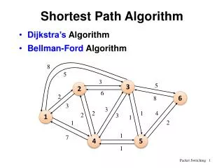
Bellman-Ford Example • Choose v3 as the source • Iteration 1: labels = [4, , 0, 6, 3], Ph = [v3, x, v3, v3, v3] • Iteration 2: labels = [4, 7, 0, 4, 3], Ph = [v3, v1, v3, v5, v3] • Iteration 3: labels = [4, 6, 0, 4, 3], Ph = [v3, v4, v3, v5, v3] • Iteration 4: labels = [4, 6, 0, 4, 3], Ph = [v3, v4, v3, v5, v3] Converged!
Where’s the Path and Costs? • What does the label Dk(s,v) mean? • The minimum cost from the source to node v in k steps. • When the algorithm converges then Dk(s,v) is the minimum cost regardless of steps • How do I find the shortest path • Walk back through the previous hop list to the source. • Example Ph = [v3, v4, v3, v5, v3] , source is v3 • v1: Path {v1, v3} • v2: Path {v2, v4, v5, v3} • v3: Source • v4: Path {v4, v5, v3} • v5: Path {v5, v3}
Example Bellman-Ford Results • Produces a tree of shortest paths from the source. • Note that this won’t necessarily be a minimum weight spanning tree. This is a different algorithm than that used for spanning trees in bridges.
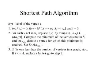
The Dijkstra’s Algorithm (used in OSPF) • Choose the source node, s. • We will find the shortest path from this node to all other nodes. • Let w(j, v) be the link weight from node j to node v. Denote the list of previous hop nodes by Ph, each node except the source will have one previous hop node from the source. Let V be the nodes of the graph and T a set of nodes that we construct. • Initialization • Set T = {s}. D(s,s) = 0, for v s, D(s, v) = w(s, v). • Repetition Step (while T V) • find u T such that D(s, u) <= D(s, v) for all v T; • add the node u to T and update the labels as follows • for all v T (updated) if D(s, v) > D(s, u) + w(u, v) then update label D(s, v) and previous hop, i.e., D(s, v) = D(s,u) + w(u,v) and previous hop for node v = u.
In Python Use a dictionary indexed by nodes for distance and previous hop Working set of nodes whose distance is not finished being minimized Main iteration loop. Assumes there will be a path from source to each node Finds the node in V with smallest distance to source Update step for distance and previous hop
Dijkstra Example • Choose v1 as the source, T = {v1} • Step 0: labels = [0, 3, 4, , ], Ph = [v1, v1, v1, x, x], T = {v1, v2} • Step 1: labels = [0, 3, 4, 5, ], Ph = [v1, v1, v1, v2, x], T={v1,v2, v3} • Step 2: labels = [0, 3, 4, 5, 7], Ph = [v1, v1, v1, v2, v3], T={v1, v2, v3, v4} • Iteration 4: labels = [0, 3, 4, 5, 6], Ph = [v1, v1, v1, v2, v4], T={v1, v2, v3, v4, v5} Finished!
Where’s the Path and Costs? • What do the labels D(s,v) mean? • When we add a node v to the set T then D(s,v) is the minimum cost. • If we are only interested in the path from s to v then we can stop the algorithm at this point (unlike Bellman-Ford where we had to continue iterating) • How do I find the shortest path? • Walk back through the previous hop list to the source. • Example Ph = [v1, v1, v1, v2, v4], source is v1 • v1: source • v2: Path {v2, v1} • v3: Path {v3, v1} • v4: Path {v4, v2, v1} • v5: Path {v5, v4, v2, v1} Much easier with Python dictionaries for distance and next hop:
Example Dijkstra Results • Produces a tree of shortest paths from the source. • Note that this won’t necessarily be a minimum weight spanning tree. This is a different algorithm than that used for spanning trees in bridges. Bellman-Ford and Dijkstra should give the same results (except for different handling of ties in an implementation).
Widest Paths? • What if we are concerned about bandwidth as much as cost, delay, or reliability? • Can we find a method like Bellman-Ford or Dijkstra? • M. Pollack, “The Maximum Capacity through a Network,” Operations Research, vol. 8, no. 5, pp. 733–736, Sep. 1960.
Widest Path via Dijkstra’sAlgorithm • Choose the source node, s. • We will find the widest path from this node to all other nodes. • Let c(j, v) be the link capacity from node j to node v. Denote the list of previous hop nodes by Ph, each node except the source will have one previous hop node from the source. Let V be the nodes of the graph and T a set of nodes that we construct. • Initialization • Set T = {s}. C(s,s) = ∞, for v s, D(s, v) = c(s, v). • Repetition Step (while T V) • find u T such that C(s, u) >= C(s, v) for all v T; • add the node u to T and update the labels as follows • for all v T (updated) if C(s, v) < min( C(s, u), c(u, v) )then update label C(s, v) and previous hop, i.e., C(s, v) = min(C(s,u), c(u,v)) and previous hop for node v = u.
Widest Path via Python Use dictionaries indexed by nodes for capacity and previous hop Working set of nodes whose capacity is not finished being maximized Main iteration loop. Assumes there will be a path from source to each node Finds the node in V with biggest capacity to source Update step for capacity and previous hop
Example Widest Path Results Shortest Paths from v1 for comparison
K-shortest Paths • We need more path choices! • Only concerned with “loopless paths” in data networks • Otherwise we’d just be wasting bandwidth resources • References • https://en.wikipedia.org/wiki/K_shortest_path_routing • J. Hershberger, M. Maxel, and S. Suri, “Finding the k shortest simple paths: A new algorithm and its implementation,” ACM Trans. Algorithms, vol. 3, no. 4, p. 45, 2007.
Performance of k-shortest paths • Yen 1971 • O(kn(m+nlog n)) • https://en.wikipedia.org/wiki/Yen%27s_algorithm • Katoh 1982 • O(k(m + n log n)) • We’ll just use my “simplistic” implementation of Yen’s algorithm • It’s based on section 4.1 (but not optimized) of: • E. Q. Martins and M. M. Pascoal, “A new implementation of Yen’s ranking loopless paths algorithm,” Quarterly Journal of the Belgian, French and Italian Operations Research Societies, vol. 1, no. 2, pp. 121–133, 2003. • Available free from: https://estudogeral.sib.uc.pt/jspui/bitstream/10316/7763/1/obra.pdf
K-shortest paths • How does it work? • Starts with the shortest path • Then looks at various “detours” • Complications: • How to make sure you look at the right set of “detours” • How to avoid repeating the same “detours” • How to be space efficient • Not easy! • Lucky for us others have done the work to make this efficient ☺
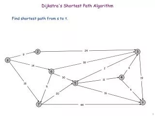
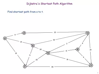
Example Network Find 20 shortest paths from n3 to n21
Example • [{"capacity":10,"cost":291.9,"nodeList":["n3","n4","n6","n13","n21"]}, • {"capacity":10,"cost":316.1,"nodeList":["n3","n4","n8","n7","n13","n21"]}, • {"capacity":10,"cost":324.3,"nodeList":["n3","n4","n6","n7","n13","n21"]}, • {"capacity":10,"cost":334.4,"nodeList":["n3","n2","n4","n6","n13","n21"]}, • {"capacity":10,"cost":343.9,"nodeList":["n3","n4","n8","n7","n14","n13","n21"]}, • {"capacity":10,"cost":352.1,"nodeList":["n3","n4","n6","n7","n14","n13","n21"]}, • {"capacity":10,"cost":358.7,"nodeList":["n3","n2","n4","n8","n7","n13","n21"]}, • {"capacity":10,"cost":366.8,"nodeList":["n3","n2","n4","n6","n7","n13","n21"]}, • {"capacity":10,"cost":372.1,"nodeList":["n3","n4","n8","n7","n14","n22","n21"]}, • {"capacity":10,"cost":380.2,"nodeList":["n3","n4","n6","n7","n14","n22","n21"]}, • {"capacity":10,"cost":386.5"nodeList":["n3","n2","n4","n8","n7","n14","n13","n21"]}, • {"capacity":10,"cost":394.6,"nodeList":["n3","n2","n4","n6","n7","n14","n13","n21"]}, • {"capacity":10,"cost":395.4,"nodeList":["n3","n4","n8","n7","n6","n13","n21"]},
Link use in 20 shortest paths Find 20 shortest paths from n3 to n21