MAGIC hyperspectral observations for studying cloud properties

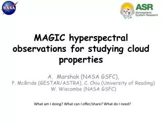
1. MAGIC hyperspectral observations for studying cloud properties Marshak (NASA GSFC), P. McBride (GESTAR/ASTRA), C. Chiu (University of Reading) W. Wiscombe (NASA GSFC) What am I doing? What can I offer/share? What do I need?

2. 'Permanent' hyperspectral instruments

3. Field deployed hyperspectral instruments

4. Multichannel instruments (overlapping with hyperspectral only)

5. FOV 2.8o Spectral range: 350-1700 nm Frequency 1 Hz Solar Spectral Flux Radiometer (SSFR)

6. Radiation Instruments @ MAGIC From Ernie’s MAGIC slide show

7. Consistency between different instruments This is 500 nm; there are some issues yet for 1600 nm

8. Inseparability of cloudy and clear skies under partial cloud cover (from Charlson et al., 2007) Albedo pdfs from LES of trade Cu and Sc clouds average of the BOMEX (~10% cloud cover) and ASTEX (overcast) fields; clear and cloudy contributions are nicely separated for ATEX trade Cu (~50% cloud cover), with the albedos from clear and cloudy portions inseparable “The existence of partly cloudy regions and the fact that the clear-cloudy distinction is ambiguous and aerosol dependent raise the possibility that the conventional expression may lead to errors.”(Charlson et al., 2007)

9. Twohy et al. (2009) estimated that “the aerosol direct radiative effect as derived from satellite observations of cloud-free oceans to be 35–65% larger than that inferred for large (>20 km) cloud-free ocean regions.” Chand et al. (2012) found a 25% enhancement in AOT between CF 0.1-0.2 and CF 0.8-0.9. This “enhancement is consistent with aerosol hygroscopic growth in the humid environment surrounding clouds.”

10. Our goal is interpret spectral radiative measurements in terms of aerosol and cloud properties in the transition zone in fully 3D cloud situations. • What do we expect to achieve? Using the spectral methods applied to MAGIC shortwave spectrometer measurements, we will be able to: • understand sources of particle changes ranging from aerosols swelling in humid air, and the detrainment of cloud-processed particles into the cloud-free environment, to the presence of undetected clouds;
 • distinguish between aerosol particles and weak cloud elements; • test the hypothesis of cloud inhomogeneous mixing in a new way. • As a result, • we expect to improve the estimates of aerosol radiative forcing and aerosol indirect effects as a function of cloud and aerosol microphysical properties

11. Spectral-invariant hypothesis

12. Radiative transfer calculations Use SBDART (1D) to calculate zenith radiance • 400-2200 nm with 10 nm resolution Atmosphere • mid-latitude summer • 3 cm water vapor column Aerosol • 0.2 – 1 optical depth at 550 nm (rural) • 80% relative humidity Cloud • 0-4 cloud optical depth (at 550 nm) • 1 km altitude from Chiu et al.,ACP2010

13. SBDART model spectra: cloud opt depth from 0 to 4 SZA = 45o reff = 6 µm AOD = 0.3 Vegetated surface

14. SBDART model: spectra omitting absorption bands (l), spectral-invariant plot (r) zooming in on red-box regions in next slide

15. SBDART model: short spectra omitting 0.9-1 µm (l), spectral-invariant plot (r)

16. Publication: McBride P.J., A. Marshak, J.C. Chiu, K.S. Schmidt, Y. Knyazikhin, E.R. Lewis, W.J. Wiscombe, 2014. Studying the cloud particle size in the cloud-clear transition zone with surface-based hyperspectral observations. J. Geoph. Res. (submitted, April 2014). The paper uses MAGIC data as an example to show that changes in the effective radius (increase or decrease) can be successfully determined using the intercept in the NIR wavelengths

17. MAGIC July 15 SSFR data

18. Cloud transition zone Retrieve qualitative cloud properties in the cloud transition zone usingaand b.

19. Modeled slope and intercept 400 - 870 nm 1530 -1660 nm The black contours are % of cloud absorption at 1600 nm calculated with SBDART τclear=0.0

20. Cloud entrainment Slide courtesy of Greg McFarquhar

21. Transition zone from MAGIC

22. HSRL data

23. Known cloudy 01:08:30 Known clear 01:19:30

24. Known cloudy 22:07:00 Known clear 22:18:00

25. Known cloudy 23:24:30 Known clear 23:25:30

26. Summary There are several shortwave (hyper)spectral instruments @ MAGIC (SAS-ze, FSSR, FRSR, Cimel). The spectral observations are used (by our ASR team) to study aerosol and cloud properties in the transition zone in fully 3D cloud situations. A new spectral technique has been developed and tested with RT simulations; it has been applied to MAGIC data on a case-by-case basis. There are many (unresolved) issues that require more analysis; we are not yet ready to apply it to all MAGIC spectral data automatically to get the TZ statistics as a function of aerosol and cloud features.

27. Cloud property retrievals

28. Cloud property retrievals

29. Zenith radiance spectra Taken at 22 and 44 s from cloud edge Time series of the ratio to 500 nm

30. Unknown “known clear” 400 - 870 nm 1530 -1660 nm τclear=0.1