WINDOWING AND CLIPPING
330 likes | 381 Views
Learn about clipping in computer graphics, from point to polygon clipping techniques. Explore Cohen-Sutherland Line Clipping Algorithm and Sutherland-Hodgman Polygon Clipping Algorithm step by step.

WINDOWING AND CLIPPING
E N D
Presentation Transcript
Points to cover • Clipping • Line clipping • Polygon clipping • Normalized transformation • Viewing transformation
Clipping • Clipping refers to the removal of part of a scene. • Any procedure which identifies that portion of a picture which is either inside or outside a region is referred to as a clipping algorithm or clipping. • The region against which an object is to be clipped is called clipping window. Usually it is rectangular in shape. • Window : it is the selected area of the picture. • Following are the graphics primitives that we are going to study under clipping: • point clipping • line clipping • polygon clipping
Line Clipping Before clipping After clipping
Space is divided into regions based on the window boundaries Each region has a unique four bit region code Region codes indicate the position of the regions with respect to the window 3 2 1 0 above below right left Region Code Legend Cohen-Sutherland: World Division
Cohen-Sutherland Algorithm (Xmax,ymax) (Xmin,ymin) Region outcodes
Cohen-Sutherland: Labelling • Every end-point of the line is labelled with the appropriate region code Three cases : Case1: Lines inside the window : not clipped Case2: lines outside the window : Take AND operation of the outcodes of the end points of the line. If answer of AND operation is non zero means line is outside the window and hence discard those lines. Case3 : lines partially inside the window :Lines for which the AND operation of the end coordinates is ZERO . These are identified as partially visible lines.
Case3: Other Lines These lines are processed as follows: • Find the intersection of those lines with the edges of window. • We can use the region codes to determine which window boundaries should be considered for intersection.eg: region code 1000 then line intersects with TOP boundary. Find intersection with that boundary only. • Check other end of the line to get other intersection. • Draw line between calculated intersection. Intersections are calculated as y coordinate of the intersection point with a vertical boundary can be calculated as y = y1 + m(x – x1), x = xmin or xmaxand m = ( y2 – y1) / ( x2– x1) x coordinate of the intersection point with a horizontal boundary can be calculated as x = x1 + (y – y1) / m , y= yminor ymaxand m = ( y2 – y1) / ( x2 – x1)
Algorithm • Read two endpoints of the line say P1 (x1,y1) and p2(x2,y2) • Read two corners of the window (left –top ) and (right-bottom) say (Wx1,Wy1) and (Wx2, Wy2) • Assign the region codes to the end co-or of P1. • Set Bit 1 – if (x<xwmin) • Set Bit 2 – if (x >xwmax) • Set Bit 3 – if (y<ywmin) • Set Bit 4 – if (y<ywmax) • Apply visibility check on the line.
Algorithm Conti… 5. If line is partially visible then- • If region codes for the both end points are non-zero , find intersection points p1’ and p2’ with boundary edges by checking the region codes. • If region code for any one end point is non-zero then find intersection point p1’ or p2’ with the boundary edge. 6. Divide the line segments considering the intersection points. 7. Draw the line segment 8. Stop.
Polygon Clipping Issues – Edges of polygon need to be tested against clipping rectangle May need to add new edges Edges discarded or divided Multiple polygons can result from a single polygon
Sutherland-Hodgman Polygon Clipping Algorithm • A technique for clipping areas developed by Sutherland & Hodgman • Put simply the polygon is clipped by comparing it against each boundary in turn. Clip Left Original Area Clip Right Clip Top Clip Bottom
Sutherland-Hodgeman Clipping Input/output for algorithm: • Input: list of polygon vertices in order. • Output: list of clipped polygon vertices consisting of old vertices (maybe) and new vertices (maybe) Sutherland-Hodgman does four tests on every edge of the polygon: • Inside – Inside ( I-I) • Inside –Outside (I-O) • Outside –Outside (O-O) • Outside-Inside(O-I) Output co-ordinate list is created by doing these tests on every edge of poly.
inside outside inside outside inside outside inside outside p s p s p s p s Save p Save I Save nothing Save I and P Sutherland-Hodgeman Clipping Edge from S to P takes one of four cases: I
Sutherland-Hodgeman Clipping Four cases: • S inside plane and P inside plane Save p in the output-List • S inside plane and P outside plane Find intersection point i Save i in the output-List • S outside plane and Poutside plane Save nothing • Soutside plane and P inside plane Find intersection point i Save i in the output-List, followed by P
Algorithhm • Read polygon vertices • Read window coordinates • For every edge of window do • Check every edge of the polygon to do 4 tests • Save the resultant vertices and the intersections in the output list. • The resultant set of vertices is then sent for checking against next boundary. • Draw polygon using output-list. • Stop.
Generalized clipping • We have used four clipping routines; one for each boundary. But these routines are identical. They differ only in their tests for determining whether a point is inside or outside the boundary. • Can we make it general ?? • It is possible to write one single routine and pass information about boundary as parameter. This change allows to clip along any line(not just horizontal or vertical boundaries).
Such general routine can be then used to clip along an arbitrary convex polygon. Fig :A window with 6 clipping boundaries
normalized coordinates • Different display devices have different screen sizes and resolutions, which is measured in pixels. • Picture on a screen with high resolution appears small in size, where as same pic on screen with less resolution appears big in size. • To avoid this we make our program device independent. • So picture coordinates have to be represented in some units other than pixels. • Device independent units are called as Normalized device coordinates. • In this screen measures 1 unit wide and 1 unit length.
Transformation to normalized coordinates • Interpreter is used to convert normalized co-ordinates into device co-ordinates. A simple linear formula is used for this. x = xn * Xw y = yn * Yw Where : x= actual device x co-or y= actual device y co-or xn = Normalized x co-or yn = Normalized y co-or Xw =Width of actual screen in Pixels Yw = Height of actual screen in Pixels
Viewing Transformation • An image is defined in a world coordinate system, WCS i.e. Using Cartesian coordinate system. • World Coordinate system: application-specific • Example: drawing dimensions may be in meters, km, feet, etc. • When picture is represented on display device,it is measured in physical device coordinate system(PDCS) corresponding to the display device. • Viewing Transformation: Mapping of coordinates is acheived with the use of coordinate transformation i.e. Maps picture coordinates in the WCS to display coordinates in PDCS.
Clipping Window Viewport • WCS is infinite in extent and device display area is finite. • A world coordinate area selected for display is called a window. ( defines what to display) • An area on a device to which a window is mapped is called viewport. ( defines where to display.)
Window to viewport coordinate transformation • Would like to: Specify drawing in world coordinates Display in screen coordinates Need some sort of mapping Called Window-to-viewport mapping Basic W-to-V mapping steps: Define a world window Define a viewport Compute a mapping from window to viewport
Window to viewport coordinate transformation • Fig shows mapping of object from window to viewport. • A point at (xw , yw ) in window is mapped into position (xv , yv ) in the associative viewport.
Scaling factors: Window to viewport coordinate transformation • To maintain relative replacement in viewport as in window we require, Solving these equations for viewport position xv = xvmin + ( xw – xwmin ) sx yv = yvmin + ( yw – ywmin ) sy Where
Window to viewport coordinate transformation • Mapping of window to viewport require following transformations • Scaling using fixed point position of (xwmin,ywmin) that scales the window area to the size of viewport area. • Translation : translating scaled window area to the position of viewport area. Workstation Transformation: Transformation of object description from normalized coordinates to device coordinates. It is accomplished by selecting a window area in normalized space and viewport area in coordinates of display device.