Bottom up: Diffuse porous flow OK, prefer Wark et al. (for now) field evidence

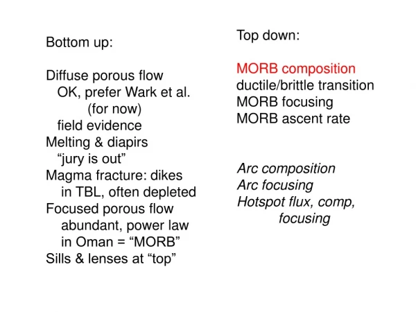
1. Top down: MORB composition ductile/brittle transition MORB focusing MORB ascent rate Arc composition Arc focusing Hotspot flux, comp, focusing Bottom up: Diffuse porous flow OK, prefer Wark et al. (for now) field evidence Melting & diapirs “jury is out” Magma fracture: dikes in TBL, often depleted Focused porous flow abundant, power law in Oman = “MORB” Sills & lenses at “top”

2. Plate driven upwelling of the mantle beneath oceanic spreading ridges drives decompression melting, and there are many aspects of this process that scientists understand well and agree upon. In this way, ridge magmatism provides a good starting point for concentrating on other, less well understood aspects of melt transport and crustal formation.

3. Summary diagram showing results of experimental melt compositions in equilibrium with mantle peridotite compositions, in terms of pressure versus SiO2 in the melt. This slide is a bit out of date, and only includes experiments up to about 1993, but the overall picture has not changed since then. (References for this compilation in Kelemen et al., Nature 1992 and Kelemen, CMP 1995). Also shown is the range of SiO2 contents observed in primitive (Mg# > 60%) mid-ocean ridge basalt (MORB) glasses from the Mid-Atlantic Ridge (MAR) and East Pacific Rise (EPR). The SiO2 contents of primitive MORB glasses are much lower than for melts in equilibrium with the mantle immediately beneath oceanic crust, at about 2 kb. Instead, the low SiO2 contents of these glasses indicate that, on average, they last equilibrated with upper mantle peridotite at more than 7 kb. The lower end of the MORB SiO2 range indicates last equilibration with mantle peridotite at an average pressure of 15 kb or more.

4. This diagram, from Braun & Kelemen, G-cubed 2003, makes the same point as the previous slide, but for more chemical components. The triangles show two pseudo-ternary phase diagrams for melting of peridotite, one projected from normative plagioclase onto the “plane” olivine-cpx-SiO2, and the other projected from normative cpx onto the “plane” olivine-plagioclase-SiO2. Bl;ue curves show the positions of olivine-cpx, olivine-opx, and opx-cpx saturation as a function of pressure in kilobars. Where the three curves meet is the melt composition in equilibrium with residual peridotite containing olivine, opx, cpx and spinel, +/- plagioclase, +/- garnet. We used the projection scheme and estimated periidotite melt compositions from Elthon, Am Min 1983, and Elthon, in Saunders & Norry ed., Magmatism in the Ocean Basins, GSA Spec. Pub., 1989.

5. linear dissolution rates for minerals in basalt, 5 to 30 kb 1500°C 1250°C orthopyroxene 10 cm/yr 1 cm/yr Summary diagram from Brearley & Scarfe, J Petrol, 1986, showing linear dissolution rates of minerals in undersaturated basaltic melt as a function of temperature; this paper reviewed results from Kuo & Kirkpatrick and Zhang et al. as well as Brearley & Scarfe’s own work. Thermodynamic treatments of these data are available in papers by Kelly Russell and co-workers (e.g., Edwards & Russell, Chem Geol 1996). Orthopyroxene dissolution rates are highlighted using the shaded field, and are greater than 0.1 meters per year over the temperature range from 1250 to 1500°C. These are very rapid rates, by geological standards, and indicate that basaltic melt ascending through opx-bearing peridotite by porous flow (melt fractions less than 30%) could not escape dissolution of, and saturation with, opx. Thus, we can infer from the primitive MORB compositions illustrated in the previous two sides, together with the kinetic data presented here, that primitive MORB does not rise through the upper ~ 40 km of the mantle via porous flow through opx-bearing peridotite.

6. √ There are essentially two ways that primitive MORB could rise through the shallow mantle without equilibrating with (very abundant) opx-bearing peridotite. One is very rapid ascent in narrow, melt filled fractures, and the other is much slower porous flow through relatively wide, opx-free dunites.

7. To remind you, here is our schematic cross section of the Oman ophiolite mantle section. Dikes, formed by melt in fractures, are present but formed off axis, transported cooling magmas, and do not have compositions in equiibrium with the melts that formed the oceanic crust. On the other hand, much larger dunites within mantle peridotite were deformed along with the peridotite, and so did form on axis in the melting region beneath the Oman spreading ridge.

8. Again, to remind you, dunites in mantle peridotites worldwide preserve contact relationships indicative of their origin via dissolution of pyroxenes from peridotite host rocks, together with formation of a slightly smaller amount of olivine, in olivine-saturated melt moving by focused porous flow through residual mantle peridotite. While we cannot rule out the presence of “cryptic cracks” in the centers of dunites, which have disappeared without a trace, we choose to assume that no cracks were present unless they are required by observations. The reasoning behind this assumption will be made clearer in the following slides.

9. again, a reminder that we cannot rule out “cryptic cracks” based on field observations alone

10. In slowly evolving “two phase flow” of buoyant melt through viscous, porous peridotite, the maximum possible pressure difference between melt in pores and the solid matrix is the product of the density difference between melt and solid, the gravitational constant, and the compaction length, where the compaction length is related to the square root of the product of permeability , bulk or shear viscosity - whichever is larger, and the reciprocal of the melt viscosity. This pressure limit applies because the viscous solid matrix is deformable, and if the pressure difference begins to exceed this maximum value, the solid will simply “decompact” to relieve the overpressure. To produce a “magma fracture” via buoyancy forces, the pressure difference between melt and solid has to exceed a yield stress for partially molten peridotite, which Kelemen et al., Phil Trans Roy Soc London estimated might be ~ 5 to 50 MPa based on (poor, approximate) experimental data.

11. The maximum possible pressure difference between melt and viscously deforming peridotite will only develop beneath an “obstruction in the flux”, as shown in many papers in the late 1980’s and early 1990’s, perhaps most elegantly by Spiegelman, J. Fluid Mechanics, 1993a,b. Here is an example, calculated by Marc Spiegelman, that illustrates this. The righthand graph shows an imposed porosity distribution, in which the porosity decreases discontinuously from 1% to 1/2% halfway up a 100 km, 1D column of olivine + melt. The viscosity and permeability are such that the compaction length in this example is 10 km. The middle graph shows pressure in the column, plus - in red field - 10 times the excess pressure in melt - solid. The righthand graph shows the excess pressure, pressure in melt - pressure in solid, in MPa as a function of height. As you can see, if there were a big obstruction in the flux, then an excess pressure of 50 MPa could develop in the melt, which might be sufficient to cause magma fracture. The excess pressure is appreciable over a distance of about one compaction length (here, 10 km) beneath the obstruction, and a somewhat shorter distance above the obstruction.

12. However, we contrast the conditions in the previous slide, and in the lefthand graph here, with the conditions preducted for steady state porosity in an upwelling, melting column of mantle peridotite, as would be present beneath a mid-ocean ridge, in the righthand graph. As you can see, in the 1D steady state approximation, porosity is predicted to increase upward, and there are no obstructions in the flux. Thus, no magma fractures are expected to originate within such a structure. As shown by Spiegelman (JFM 1993a,b) and Khodakovskii (Univ. Toulouse PhD thesis), perturbations to the structure on the right decay with increasing height, because the permeability increases with increasing height. Thus, even if melt rich bands appeared relatively rapidly at the bottom of the melting column, the resulting porosity waves (with downstream “obstructions” above and below each wave) would get smaller and smaller upward. For these reasons, we think magma fracture is unlikely within the partially melting, upwelling mantle beneath mid-ocean ridges.

13. So … again … we are going to proceed from field evidence that definitely does support the hypothesis that melt migrates by focused porous flow in dunites that formed by replacing host peridotite. We cannot rule out the presence of magma fracture, but for the reasons summarized in the past few slides we are going to assume that magma fracture does not occur in the melting region beneath ridges, except near the top, close to the base of the conductive boundary layer.

14. Instead, we have developed a conceptual model for melt transport in high porosity dissolution channels that form via the reactive infiltration instability. To remind you, this slide is a general illustration of how elongate dissolution channels can form where a fluid solvent migrates by porous flow through a partially soluble porous matrix. There is positive feedback between permeability, permitting increased flux of the solvent, and dissolution, increasing the local permeability and porosity, which leads to the exponential growth of high porosity dissolution channels in the primary direction of fluid flow. The earliest literature on this “reactive infiltration instability” were by Chadam et al., J. App. Math., 1986; Ortoleva et al., Am J Sci, 1987; Steefl & Lasaga, ACS Symposium Series, 1990.

15. This illustration, from Kelemen et al., JGR 1995, shows a tank experiment in which we passed fresh water (think, “olivine-saturated melt”) from top to bottom through a mixture of glass balls (think “olivine) and salt (think “pyroxene”). Over time, salt free, high porosity dissolution channels formed and grew downward as a result of salt dissolution.

16. The largest channels in the experiment lengthened exponentially as a function of time, while small channels decayed away as the flow was “captured” by their larger neighbors. The aspect ratios of the channels reflected the balance between advective flow times down the increasingly long channel and diffusive exchange times laterally from salt-rich regions into the channels, as predicted by, e.g., Steefel & Lasaga, 1990. This balance is maintained because the channels can only grow longer while “fresh”, undersaturated water can flow from one end to the other.

17. Here is another simple experiment, in this case a numerical one from Einat Aharonov, published in Kelemen et al., JGR 1995. Prior to that paper, all treatments of the reactive infiltration instability started with an assumed solution front, in which undersaturated fluid enters a partially soluble porous matrix across a sharp front. We wondered how such a sharp front could develop in the mantle, or in any other geological system for that matter. In this experiment, fluid is modeled as small particles which interact elastically. There is a “pressure gradient”, driving these particles from the bottom to the top, and the small arrows show the local, average, velocity vectors for the particles. The squares are solid particles. It has been shown that this kind of “lattice gas” and “lattice Boltzmann” model can reproduce Darcy’s Law and other, more complicated empirical relationships for porous flow (e.g., Aharonov & Rothman, GRL 93). In this experiment, when a fluid particle collides with a solid particle the solid particle can “dissolve” and become part of the fluid. There is a solubility gradient in the model domain, which can be conceptualized as follows: particles entering the box are “red”; particles that detach from the solid and become part of the fluid are “blue”. The solubility in some part of the model can be defined as the probability that a solid particle will detach, which is a function of the local concentration of blue/red. Here, the solubility increases downstream (upward). The solubility gradient is imposed by requiring that the saturation value of blue/red is higher and higher upward. Initially, the fluid is saturated in solid everywhere in the model (detachment probability = 0 everywhere). However, as fluid flows upward, it has to dissolve solid particles in order to remain saturated. Even if the reaction kinetics are “fast” so that the probability of detachment increases very rapidly as blue/red departs from the equilibrium value, dissolution will occur as a result of flow through the solubility gradient. To complete this experiment, we left out one large solid particle in the middle of the model domain, in the sixth row from the top. As you can see, a large dissolution channel develops, both upstream and downstream from the missing particle. Fluid flowing through the center of this channel remains strongly undersaturated in the solid, and so the downstream end of the channel becomes a sharp solution front, even though we started from local equilibrium everywhere. Another thing to see here is that, despite the very simple physics in this model, the dissolution channel is “underpressured” at the bottom, so that fluid flow coalesces toward the channel, and the channel is overpressured at the top where it impinges on un-dissolved solid particles, so fluid flow diverges.

18. Here is a slightly more complicated experiment, performed by Mike Braun, Jack Whitehead and me. We probably won’t ever publish these results, because they replicate to a large degree very elegant experiments by Tait & Jaupart, JGR 1992 and Tait et al., Nature 1992. In our experiment, we again used a kind of pseudo-2D geometry, a narrow tank much wider and taller than it is thick. The tank was filled with powdered ammonium chloride + water, and cooled from below. The solubility of ammonium chloride in water is very strongly correlated with temperature, so ammonium chloride precipitates near the bottom of the tank, and dissolves higher up. The density of ammonium-chloride-rich aqueous solutions is much more strongly dependent on composition than on temperature, so cold, NH4Cl-poor solutions are much less dense than hotter, NH4Cl-rich solutions. As a consequence, there is compositional convection in the tank, with cold ammonium chloride rich solutions rising from the base, and warm, ammonium chloride poor solutions descending to the bottom. As the relatively “fresh” water rises from the bottom of the tank, because thermal diffusion is faster than chemical diffusion, the water warms and begins to dissolve surrounding ammonium chloride crystals. Eventually, as you can see in this shadow-graph, the upflow is organized into very highly focused, high porosity chimneys in which all the ammonium chloride has been dissolved. These are separated by lower porosity regions in which diffuse downwelling of cooling, crystallizing water precipitates new ammonium chloride crystals. Although this geometry is somewhat different from what we envision in the mantle - because of the return flow in the tank - this experiment provides an exceptionally clear and graphic illustration of the reactive infiltration instability.

19. Our basic hypothesis, then, is that high porosity dissolution channels form as a result of the reactive infiltration instability, via dissolution of pyroxenes and precipitation of a smaller mass of olivine, increasing the porosity and permeability. Eventually, within these channels, all of the pyroxene is exhausted, forming high porosity dunite conduits. Because the permeability of olivine-only dunite is higher than that of olivine+pyroxene peridotite, melt will continue to flow mainly within the dunite conduits. Once dunites are sufficiently wide (ca 1 meter wide, see Braun & Kelemen, G-cubed 2002), melt flowing through the dunites will not maintain equilibrium with pyroxenes in surrounding peridotite. In this way, melts recording equilibrium with peridotite at an average pressure of ~ 15 kb flow through the upper ~ 45 km of the melting region without equilibrating with pyroxenes in the shallow mantle.

20. flux/channel  width Aharonov et al., JGR 1995, formally extended the mathematical formulation of the reactive infiltration instability to include (a) formation of high porosity dissolution channels during porous flow with solubility gradients rather than a solubility front, and (b) channel formation in a viscously deforming porous medium. We showed, with subsequent elaboration by Spiegelman et al., JGR 2001, that dissolution channels are enhanced, rather than suppressed, by viscous deformation. We found that channels in this system have a preferred wavelength, and that this wavelength increases with increasing melt flux (velocity * porosity). Thus, we imagined that an initial set of channels would grow on a very small scale, with a resulting increase in the mean velocity and flux of the melt. This, in turn, would favor growth of larger, more widely spaced channels, and so on. Thus, we drew the diagram in the lower left, which we call “Einat’s Castle” after Einat Aharonov, showing a cascading network of increasingly large channels, without really being sure whether the vertical dimension was space, or time, or both. Kelemen et al., G-cubed 2000, noted that Einat’s castle yields a simple power law relating frequency to flux/channel, since at every junction the number of channels decreases by a factor of 2 and the flux per channel doubles. If, in such a coalescing network, the width/channel is proportional to the flux/channel to some power (as in Einat’s Castle), this structure will also have a power law relationship between frequency and width.

21. We then moved to a more complex numerical model the formation of dissolution channels in a viscously deforming, partially soluble porous medium. This diagram, from Spiegelman et al., JGR 2001, illustrates the model setup, which is conceptually very similar to the analogue and lattice gas experiments illustrated earlier. A solvent flows into the bottom of the model domain, and out the top. Initially, the solvent is at local equilibrium everywhere in the model domain, but there is a solubility gradient increasing from bottom to top, so that the solvent has to dissolve the soluble solid phase in order to maintain equilibrium as it moves upward. “Two phase flow” of the liquid and the viscous solid are modeled using the formulation of McKenzie, J Petrol 1984, as implemented by Spiegelman (e.g., Spiegelman & McKenzie, Nature 1987; Spiegelman, Phil Trans Roy Soc London, 1993).

22. Here we show model results for porosity evolution near the top of the model domain, as a function of distance across the model domain, illustrating the formation of high porosity channels as a function of non-dimensional time. Note that t=1 corresponds to the time for the melt or fluid to migrate one compaction length at the initial porosity of 1. Note that, unlike in models with “rigid” porous media, the intervening regions between the dissolution channels show decreasing porosity with time. It is for this reason that addition of viscous deformation in the porous matrix actually enhances, rather than damps, the reactive infiltration instability.

23. This figure, from Kelemen et al., G-cubed 2000, illustrates just one additional numerical modeling result. (Those interested should look at the paper by Spiegelman et al., JGR 2001, for more complete results). Here we’ve emphasized the structure of the dissolution channel network in a model run by dividing the porosity at any height by the mean porosity at that height. Thus, although the porosity in small diffuse channels near the bottom of the model domain is very small compared to the porosity in the much better developed channels near the top, this image shows how the channels at each height connect. You can see that the channels produced in the numerical model form a binary coalescing network very similar to Einat’s Castle. Thus, we can infer that Einat’s Castle is a stucture produced in space as a result of the reactive infiltration instability. Also, if a numerical model can “confirm” a theory based on a linear stability analysis, then we can say that the numerical model confirms our earlier hypotheses.

24. Here we look at another aspect of the coalescing channel network in the previous image. In this figure from Spiegelman et al., JGR 2001, we have plotted the number of “channels” at any height (number of regions with porosity > average at that height) versus height. As you can see, after a time of about 50, the coalescing channel network has developed. The good news, for geologists, is that despite many other transient features in the modeling results, the channel network reaches a steady state geometry, and then remains roughly constant at longer times. Thus, we might be able to observe such a network in the field, without knowing at what time a natural geological system “froze” and stopped evolving.

25. lungs Note that we are not expecting a natural channel network to look like the idealized model results, with binary coalescence of equal sized channels at every junction. Instead, we expect a lot of “side branching”, in which quite small channels entering very large ones. For this reason, we infer that a natural network might look more like this image of the arterial network in mammalian lungs, already shown in a previous lecture. However, like the deterministic fractal tree of Einat’s Castle, more complicated coalescing networks of this type generally show a power law distribution of frequency versus flux, and frequency versus width (e.g., Murray, Proc. Nat. Acad. Sci. (USA) 1926).

26. As I showed in a previous lecture, measurements of dunites within residual mantle peridotite in the Ingalls ophiolite (Kelemen et al., G-cubed 2000) and the Oman ophiolite (Braun & Kelemen, G-cubed 2002) demonstrate that dunites show a power law relationship between width and frequency, as predicted for a coalescing channel network. This result does not prove that dunites do form a coalescing network, but it is certainly consistent with that idea, and confirms a central prediction of our hypothesis.

27. Thus, based on the field relationships in the right hand diagram, informed by geochemical observations, field measurements, and theory, we construct the hypothetical dunite network in the left hand diagram, with many coalescing dunite channels converging upward toward an oceanic spreading ridge. Because the dunites form about half way up the ~ 100 km tall melting region, they preserve melt compositions in equilibrium with peridotite at an average depth of ~ 45 km.

28. There may be a lot of other analogous systems. This is a movie of a “black smoker”, a submarine hot spring associated with volcanoes along a mid-ocean ridge, with diffuse recharge, and very highly focused output. I have yet to see a good paper explaining this focusing in terms of reactive porous flow, but I suspect one could be written!

29. Hoefner & Fogler, AIChE 34, 1988 Now I’d like to digress a bit and talk about some more general features of channel formation via the reactive infiltration instability. This diagram is from a paper by Hoefner & Fogler in Am Inst Chem Eng Journal, 1988. That paper includes results from both analogue experiments, in which acid was injected into plaster cylinders, and numerical experiments like those illustrated here. In these experiments, flow velocity of a solvent through a partially soluble porous medium increases from right to left and bottom to top, while all other variables are held constant. In each panel the solvent flows through a soluble porous medium from bottom to top. In the lower right, very slow flow produces a slowly moving, planar dissolution front perpendicular to the flow direction. No channels form, because diffusion is faster than advection, so that even if there are high and low porosity variations along the front, concentration of the solute does not vary laterally, so that dissolution is no faster in high porosity regions compared to low porosity regions. As the flow rate increases, highly focused channels form and grow downstream. However, at really fast flow rates, dissolution is too slow to approach local equilibrium between fluid and solid, and so - in essence - every pore becomes a channel, and no channels are favored. Thus, channels form most markedly at intermediate flow velocities. I show this figure in order to emphasize how similar this result is to what we know about mechanical erosion. Imagine that the panels in the figure are planar surfaces of sand, onto which rain is falling. The slope, and the flow velocity of water over the surface, increases from right to left and bottom to top. At the lowest slopes, water moves very slowly and cannot displace any grains. At intermediate slopes, water in relatively low areas with relatively rapid flow can displace grains, creating channels which have low surface area/volume and so increasingly rapid flow. These channels then propagate downstream. Finally, on very steep slopes, flow is rapid everywhere, and there is little energetic difference between flow in laterally low versus high areas at a given distance downslope, so water moves in “sheet flow” over the surface.

30. This analogy can be further extended by looking at this photo, of sapping channels on a beach. I copied this photo from a catalogue for climbing equipment, and so I don’t know who took it, or where. I also want to point out that part of the photo has been electronically “faked”. The two channels on the right are identical to the two channels on the left, and the photographer or someone has simply removed the shell in the righthand pair. Anyway … sapping channels form on beaches when the tide goes out below the level of the ground water table in the sand. At this point, ground water comes to the surface, and flows down the beach. In some places, these beautiful and very simple channel networks form twice a day. For the moment, I just want you to see that the erosional channel network looks a lot like Einat’s Castle, or our numerical results, with many small channels - all active at the same time - coalescing to join a few large channels downstream.

31. Top down: MORB composition slow flow in dunites ductile/brittle transition MORB focusing MORB ascent rate Arc composition Arc focusing Hotspot flux, comp, focusing Bottom up: Diffuse porous flow OK, prefer Wark et al. (for now) field evidence Melting & diapirs “jury is out” Magma fracture: dikes in TBL, often depleted Focused porous flow abundant, power law in Oman = “MORB” Sills & lenses at “top”

32. OK, now on to something else. So far, I’ve tried to explain melt extraction from the mantle in terms of relatively slow, porous flow through dissolution channels. There is nothing in these models that would produce a lot of time dependence - there are some predictions of “porosity waves” that I haven’t talked about, but these are predicted to ebb and flow on time scales of thousands of years or more. Thus, the model I have been promoting here has no way of explaining punctuated melt transport of the type that formed this outcrop of sheeted dikes in the Oman ophiolite. John Delaney likes to call these dikes the “quantum event” of oceanic crustal formation. I used to think this was silly, but now I think it is profound. In any case, we’d like to have a theory that explains the transition from continuous, porous flow to punctuated, rapid transport in fractures.

33. Here is another simple experiment illustrated in a figure from Kelemen et al., JGR 1995. Here, Kelsey Jordahl, Jack Whitehead and I placed a circular glass plate with a small hole in the center over a circular cold plate, with a small gap between glass and cold plate. You are meant to think of the gap as melt porosity in mantle peridotite. From a constant height (constant pressure), saturated aqueous ammonium chloride solution is fed at room temperature through the central hole, from which it flows radially outward over the cold plate. Because the solubility of ammonium chloride in water is strongly correlated with temperature, the solution flowing outward over the cold plate forms ammonium chloride crystals, gradually decreasing the permeability of the gap between the glass and the cold plate. Initially, crystallization occurs diffusely over the entire surface, and water coming out the edges is cold and relatively fresh. However, quite quickly, one highly permeable pathway becomes established. This gradually becomes more and more focused, because fluid that diverges from this path slows down, cools further, and crystallizes more. As a result, the edges of the channel become increasingly impermeable, in a process analogous to formation of natural levees around a river channel. Once flow is highly focused, there is little cooling, so the water coming out the side is relatively warm and saline. However, even the fast moving fluid in a narrow channel does cool and crystallize to some extent. Ultimately, as the channel becomes “clogged” with new crystals, the fluid finds a new pathway through the walls armoring the channel, either by porous flow or by fracture. Then a new channel with armored walls forms. Ultimately, this process forms a diverging network that fills the entire disk.

34. We think the processes in the experiment shown in the previous slide may be applicable to understanding crystallization of ascending melt in pore space in mantle peridotite as it rises into the thermal plate and undergoes conductive cooling and crystallization. Here, in a figure from Kelemen & Aharonov, AGU Monograph 1998, we show the effects of cooling on the fraction of liquid for various estimated primitive mid-ocean ridge basalt (MORB) compositions, based on calculations using the MELTS thermodynamic model for silicate liquids. Most of these primitive MORB compositions are predicted to saturate in olivine at ~ 1300°C, but they do not crystallize much until they become saturated in olivine + plagioclase at about 1240°C. At this stage, the liquids are close to being “eutectic”, meaning that they crystallize to a large degree over a very narrow temperature interval. At this stage, if the melt flux is large and the cooling rate is fast, melt crystallization becomes capable of filling pore space, drastically reducing permeability, and leading to a large upstream increase in melt pressure if the incoming flux is fixed.

35. Korenaga & Kelemen, JGR 1997, provided simple scaling for processes which do, and do not, fill pore space by crystallization of cooling, crystallizing melt. The time scale for viscous compaction or decompaction in response to gradients in melt pressure is given by equation (8), above, and is the viscous compaction length divided by the melt velocity (actually, Darcy flux = velocity * porosity). The time scale for melt crystallization is given by equation (9), and is the reciprocal of the product of melt flux, the geotherm (°C/m), and the change in melt fraction with temperature (as in the previous slide). When the time scale for crystallization is shorter than that for decompaction, then pore space will fill,and melt pressure will rise upstream. When the time scale for viscous decompaction is short compared to the crystallization time, then incipient pressure rise in the melt will be accommodated by viscous expansion, increasing the total volume of the system and maintaining nearly constant porosity. Short crystallization times are favored by high melt flux (velocity), large temperature changes over a short distance, and rapid crystallization rates per °C of cooling, as for olivine + plagioclase saturated melt in the previous slide. Thus, we can expect pore space to fill as melt cools in the conductive boundary layer in areas with thin plates and high melt flux (mid-ocean ridges, and perhaps “hotspots”). In contrast, we can expect cooling melt to flow more or less readily into the conductive boundary layer in areas with thick plates and low melt flux, as in continental interiors. The latter case may be a good way of thinking about “mantle metasomatism”.

36. Some of this thinking was anticipated by Spiegelman (Phil Trans Roy Soc London 1993), who followed the proposal of Sparks & Parmentier (EPSL 1991), and modeled formation of a permeability barrier at the base of the thermal plate, above the melting region adjacent to a mid-ocean ridge. Spiegelman’s results are illustrated in the two lefthand panels here. Using the McKenzie (J Pet 1984) formulation for two phase flow, Spiegelman found that, where the crystallization rate in one compaction length, 0, was small, no permeability barrier would form, whereas at high crystallization rates, a permeability barrier forms by crystallization in pore space at the base of the thermal plate, and melt migrates in a high porosity decompaction channel which forms beneath this barrier. A more recent set of models of this same process, by Rabinowicz & Ceuleneer (EPSL 2006), is shown on the right.

37. We interpret gabbroic lenses in the crust-mantle transition zone of the Oman ophiolite in the context of these models. Thus, melt rising into the conductively cooled mantle just beneath the base of newly forming oceanic crust becomes saturated in olivine + plagioclase. At this point, the crystallization rate becomes very large, and permeability barriers develop. Immediately beneath the ridge axis, these permeability barriers - which are parallel to isotherms - are horizontal or dome shaped so that melt cannot migrate diagonally from beneath them. Instead, melt pressure begins to rise, opening melt filled lenses. Partial crystallization in these melt lenses forms the gabbroic sills that we observe

38. Qcrack Qviscous Qin Kelemen & Aharonov, AGU Monograph 1998, provided a very simple “toy model” of this process. Constant, porous flux enters a melt lens. Viscous flux out (due to pressure dependent porous flow of melt out of the lens, irreversible viscous expansion of the lens, and crystallization of melt in the lens) is less than or equal to the influx. Where the input is larger than the viscous flux out of the lens, melt pressure rises. A fracture can form at a given yield stress; when the fracture forms, it propagates to a free surface in a process that is not modeled. A given melt pressure is required to resist elastic stresses that tend to close the fracture. When the fracture width falls below some minimum value, the crack is “closed” and “healed”, and the yield stress to form a crack returns to its original value.

39. Qcrack Qviscous Qin Two steady solutions are possible. In the lefthand panel, influx is greater than viscous flow out of the lens, so a crack forms. Then, influx is sufficient to maintain the pressure required to keep the crack open, and melt flows steadily through the crack. This may be a good way to understand the continuous eruption of Kilauea volcano in Hawaii. In the righthand panel, melt pressure in the lens rises until the viscous flow out is equal to the input flux, and then the system reaches steady state.

40. Qcrack Qviscous crack forms viscous flow pressure flow in crack Qin crack heals flux out A more interesting solution lies at fluxes intermediate between the fast input that forms a permanent crack and the slow input that is balanced by viscous flow out of the lens. Here, the input is sufficient to form cracks, but not sufficient to keep them open. Under these conditions, the system is perfectly periodic, regularly forming and closing magma fractures.

41. We think this latter case may be a good way to understand the punctuated, possibly periodic, formation of dikes with very restricted range of sizes, as in sheeted dikes in ophiolites and in tectonic exposures on the sea floor.

42. In addition, Kelemen & Aharonov (AGU Monograph, 1998) proposed that periodic pressure changes in melt lenses, as a result of the periodic formation of melt-filled fractures, could shift the cotectic proportions of crystallizing minerals, developing the modal layering of minerals that is commonly seen in gabbro lenses in the crust mantle transition zone, and in lower crustal gabbros, in the Oman ophiolite.

43. Now I would like to return one last time to the analogy between the melt transport processes described in this lecture, and clastic erosion and deposition. I already mentioned the parallels between dissolution channels and erosional channels. Now I would like to focus on the regime of precipitation in pore space, as compared to deposition in “deltas”. On the right is the photo of sapping channels on a beach that I showed earlier. Note that to first order the depositional deltas in the bottom half of the photo , with their diverging flow paths, are “symmetrical” with the erosional network in the top half of the photo, with its coalescing channels. However, in detail, only one or two channels in the delta are occupied at any given time, different from the erosional network where all channels are active at once, but similar to our chemical deposition experiment where over the long term flow is diverging, but at any given time flow is tightly restricted in a single channel.