Download
1 / 74
740 likes | 854 Views
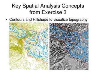
Key Spatial Analysis Concepts from Exercise 3 . Contours and Hillshade to visualize topography. Zonal Average of Raster over Subwatershed. Join. Subwatershed Precipitation by Thiessen Polygons. Thiessen Polygons Intersect with Subwatersheds Evaluate A*P Product

E N D
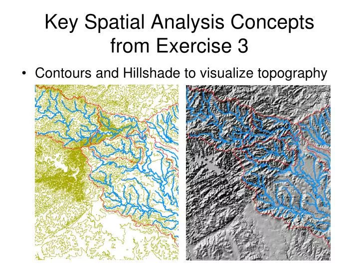
Key Spatial Analysis Concepts from Exercise 3 • Contours and Hillshade to visualize topography
Subwatershed Precipitation by Thiessen Polygons • Thiessen Polygons • Intersect with Subwatersheds • Evaluate A*P Product • Summarize by subwatershed
Subwatershed Precipitation by Interpolation • Kriging (on Precip field) • Zonal Statistics (Mean) • Join • Export
Runoff Coefficients • Interpolated precip for each subwatershed • Convert to volume, P • Sum over upstream subwatersheds in Excel • Runoff volume, Q • Ratio of Q/P
Digital Elevation Model Based Watershed and Stream Network Delineation Readings • At http://resources.arcgis.com, in the Desktop | Geoprocessing | Tool Reference | Spatial Analyst Toolbox Hydrology Toolset start from “An overview of the Hydrology tools” http://resources.arcgis.com/en/help/main/10.1/index.html#//009z0000004w000000 and read to end of Hydrologic analysis sample applications in the Hydrology toolset concepts section How to use Understanding
The Terrain Flow Information Model • Pit removal • Flow direction field derivation • Flow Accumulation • Channels and Watersheds • Raster to Vector Connection
The terrain flow information model for deriving channels, watersheds, and flow related terrain information. Pit Removal (Filling) Raw DEM Channels, Watersheds, Flow Related Terrain Information Flow Field Watersheds are the most basic hydrologic landscape elements
DEM Elevations 720 720 Contours 740 720 700 680 740 720 700 680
The Pit Removal Problem • DEM creation results in artificial pits in the landscape • A pit is a set of one or more cells which has no downstream cells around it • Unless these pits are removed they become sinks and isolate portions of the watershed • Pit removal is first thing done with a DEM
Pit Filling Increase elevation to the pour point elevation until the pit drains to a neighbor
Pit Filling Original DEM Pits Filled Pour Points Pits
80 80 74 74 63 63 69 69 67 67 56 56 60 60 52 52 48 48 Hydrologic Slope - Direction of Steepest Descent 30 30 Slope:
2 2 4 4 8 1 2 4 8 4 32 64 128 4 1 2 4 8 16 1 2 4 4 4 4 8 4 2 1 2 1 4 16 Eight Direction (D8) Flow Model
32 64 128 16 1 8 4 2 Flow Direction Grid
Flow Accumulation Grid. Area draining in to a grid cell 0 0 0 0 0 0 0 0 0 0 0 2 2 2 0 2 2 0 0 2 0 1 0 0 10 0 0 1 0 10 1 0 0 0 14 0 1 0 0 14 1 0 4 1 19 4 1 0 1 19 Link to Grid calculator ArcHydro Page 72
Stream Network for 10 cell Threshold Drainage Area Flow Accumulation > 10 Cell Threshold 0 0 0 0 0 0 0 0 0 0 2 2 0 0 2 0 2 2 2 0 0 0 1 0 0 1 10 0 0 10 0 1 0 0 1 0 0 14 0 14 4 1 0 1 1 0 4 1 19 19
1 1 1 1 1 1 3 3 3 1 1 2 1 1 11 2 1 1 1 15 2 1 5 2 20 TauDEM contributing area convention. 1 1 1 1 1 3 3 1 1 3 1 1 2 1 11 1 2 1 1 15 5 2 1 2 25 The area draining each grid cell includes the grid cell itself.
Streams with 200 cell Threshold(>18 hectares or 13.5 acres drainage area)
Watershed andDrainage PathsDelineated from 30m DEM Automated method is more consistent than hand delineation
Stream Segments 201 172 202 203 206 204 Each link has a unique identifying number 209 ArcHydro Page 74
Vectorized Streams Linked Using Grid Code to Cell Equivalents Vector Streams Grid Streams ArcHydro Page 75
DrainageLines are drawn through the centers of cells on the stream links. DrainagePoints are located at the centers of the outlet cells of the catchments ArcHydro Page 75
Catchments • For every stream segment, there is a corresponding catchment • Catchments are a tessellation of the landscape through a set of physical rules
Catchment GridID DEM GridCode 4 3 5 Vector Polygons Raster Zones Raster Zones and Vector Polygons One to one connection
Catchments, DrainageLines and DrainagePoints of the San Marcos basin ArcHydro Page 75
Catchment, Watershed, Subwatershed. Subwatersheds Catchments Watershed Watershed outlet points may lie within the interior of a catchment, e.g. at a USGS stream-gaging site. ArcHydro Page 76
Advanced Considerations • Using vector stream information (DEM reconditioning) • Enhanced pit removal • Channelization threshold selection • Computational considerations
“Burning In” the Streams Take a mapped stream network and a DEM Make a grid of the streams Raise the off-stream DEM cells by an arbitrary elevation increment Produces "burned in" DEM streams = mapped streams = +
AGREE Elevation Grid Modification Methodology – DEM Reconditioning
Carving Lower elevation of neighbor along a predefined drainage path until the pit drains to the outlet point
Carving Original DEM Carved DEM Carve outlets Pits
Filling Minimizing Alterations Carving
Minimizing DEM Alterations Original DEM Optimally adjusted Carved Pits Filled
AREA 2 3 AREA 1 12 How to decide on stream delineation threshold ? Why is it important?
Delineation of Channel Networks and Catchments 500 cell theshold 1000 cell theshold
Hydrologic processes are different on hillslopes and in channels. It is important to recognize this and account for this in models. Drainage area can be concentrated or dispersed (specific catchment area) representing concentrated or dispersed flow.
Examples of differently textured topography Badlands in Death Valley.from Easterbrook, 1993, p 140. Coos Bay, Oregon Coast Range. from W. E. Dietrich
Gently Sloping Convex Landscape From W. E. Dietrich
Topographic Texture and Drainage Density Same scale, 20 m contour interval Driftwood, PA Sunland, CA
“landscape dissection into distinct valleys is limited by a threshold of channelization that sets a finite scale to the landscape.” (Montgomery and Dietrich, 1992, Science, vol. 255 p. 826.) Lets look at some geomorphology. • Drainage Density • Horton’s Laws • Slope – Area scaling • Stream Drops Suggestion:One contributing area threshold does not fit all watersheds.
Drainage Density • Dd = L/A • Hillslope length 1/2Dd B B Hillslope length = B A = 2B L Dd = L/A = 1/2B B= 1/2Dd L
Drainage Density for Different Support Area Thresholds EPA Reach Files 100 grid cell threshold 1000 grid cell threshold
Hortons Laws: Strahler system for stream ordering 1 3 1 2 1 2 1 1 1 1 1 2 2 1 1 1 1 1 1