Download
1 / 45
450 likes | 483 Views
Explore gene identification strategies in prokaryotic and eukaryotic genomes, using Hidden Markov models. Learn about gene structures, HMM applications, and gene annotation methods.

E N D
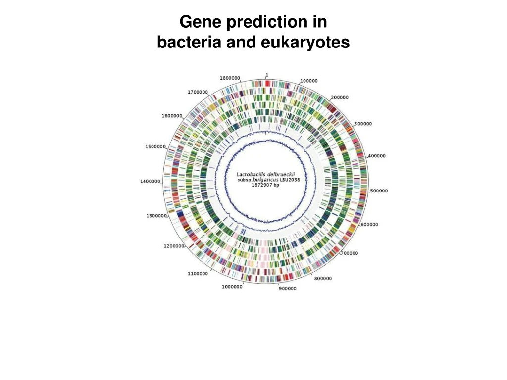
Gene prediction in bacteria and eukaryotes
Gene structure Bacteria Eukaryotes
Outline • Identification of genes in prokaryotic genomes • - Genome and gene structure • - Introduction to Hidden Markov models (HMMs) • - Example programs: GLIMMER and FGENESB • 2. Identification of genes in eukaryotic genomes • - Genome and gene structure • - Intrinsic and extrinsic approaches • - Example programs: FGENESH
Prediction of genes Typically, the first bioinformatic step after sequencing a genome is the identification and annotation of genes. Identification of the functional content of a genome. - protein encoding genes - ribosomal RNA genes (rRNA) - transfer RNA genes (tRNA) - small RNAs Gene identification is more difficult in eukaryotes than prokaryotes.
Characteristics of bacterial and archaeal genomes Gene annotation in prokaryotes (bacteria and archaea) is relatively simple compared to eukaryotes because: 1. High gene density – one gene per kilobase 2. Absence of introns 3. Very little repetitive DNA
Annotation of genes in bacteria (and archaea) Genes are most simply identified by the presence of long open reading frames (ORFs) Prokaryotic genes are often in an operon structure
Gene recognition in genomic DNA 1. Open reading frame (ORF) length An ORF is defined by a start codon and a stop codon. 5’-ATG GTG TTG TAA-3’ TAG TGA Alternative start codons in bacteria
Gene recognition in genomic DNA 2. Patterns of codon usage that are consistent with genes
Gene recognition in genomic DNA 2. Patterns of codon usage that are consistent with genes Markov models are very useful in defining the coding potential of putative protein-coding DNA sequences. e.g. GLIMMER and FGENESB
Markov chains and models A Markov model (or chain) refers to a series of observations in which the probability of an observation depends on a number of previous observations.
Markov chains and models A Markov model (or chain) refers to a series of observations in which the probability of an observation depends on a number of previous observations. The number of previous observations defines the order of the chain Fifth order Markov model are used in gene prediction For coding regions of DNA, it is well known that the probability of a given base depends on the 5 bases preceding it.
Fifth order Markov models Coding DNA sequence: * TAA-3’ * 5’-ATG M GAT D ATC I GCC A ATC I CAC H How well does the local nucleotide sequence conform to the fifth order dependencies observed in coding regions? The higher the conformity, the higher the probability the DNA sequence is protein-encoding
Hidden Markov models Hidden Markov models (HMMs) are used to provide a statistical representation of real biological processes. Genetic elements (e.g. coding or noncoding) are referred to as states
Hidden Markov models Hidden Markov models (HMMs) are used to provide a statistical representation of real biological processes. Genetic elements (e.g. coding or noncoding) are referred to as states Transition probabilities: how likely a change of state is, as one moves through the sequence
Hidden Markov models Hidden Markov models (HMMs) are used to provide a statistical representation of real biological processes. Genetic elements (e.g. coding or noncoding) are referred to as states Transition probabilities: how likely a change of state is, as one moves through the sequence Emission probabilities: each state emits a particular nucleotide with some probability
Hidden Markov models Hidden Markov models (HMMs) are used to provide a statistical representation of real biological processes. The sequence characteristics provide information on how likely a state is as one moves through the sequence. The user “sees” the nucleotide sequence being analyzed, but does not actually see the state that the base is in - hence the term “hidden” markov model.
HMMs need training sets Hidden Markov models (HMMs) are derived from training sets, where the correct structure is already known. Transition and emission probabilities are derived from training sets. The objective of training is to define a set of parameters that maximize the correct prediction for a new sequence of interest. Model parameters differ from organism to organism, therefore the success of a HMM-based method depends on how well the training set represents the sequence of interest.
Gene recognition in genomic DNA 3. A consensus sequence for ribosome binding site in the vicinity of a start codon. +13 -20 ATG 5’-ATG TAA-3’ TAG TGA In bacteria, ribosome binding site is called a Shine-Dalgarno sequence.
Gene recognition in genomic DNA 4. Homology of putative genes to other previously described genes - Genomic DNA can be searched against protein databases using blastx - Exons can be matched to cDNA sequences
Gene recognition in genomic DNA 1. Open reading frame (ORF) length 2. Patterns of codon usage that are consistent with genes 3. A consensus sequence for ribosome binding site in the vicinity of a start codon. 4. Homology of putative genes to other previously described genes Intrinsic approaches (ab initio) Extrinsic approaches
Bacterial gene prediction: GLIMMER GLIMMER is a bacterial (archaeal and viral) gene finding algorithm that uses a fifth order Markov chain. Step 1. Build a Markov model from a training set Step 2. Scan genomic DNA sequence to predict genes Criteria for gene finding: - start and stop codon - minimal length for an ORF
FGENESB: bacterial operon and gene prediction FGENESB gene prediction algorithm is based on Markov chain models of coding regions and translation and termination sites. http://linux1.softberry.com/berry.phtml
FGENESB: step by step description of annotation 1. Finds all potential ribosomal RNA genes using BLAST search against ribosomal RNA databases. 2. Predicts tRNA genes using tRNAscan-SE program
FGENESB: step by step description of annotation 1. Finds all potential ribosomal RNA genes using BLAST search against ribosomal RNA databases. 2. Predicts tRNA genes using tRNAscan-SE program 3. Initial prediction of ORFs using fifth and second order Markov models 4. Predict operons based on distance between predicted genes
FGENESB: step by step description of annotation 5. Runs BLAST for predicted proteins against COG database 6. Uses information about known neighboring gene pairs to improve operon prediction 7. Runs BLAST for predicted proteins against NCBI nr database 8. Predict promoters and terminators 9. Refine operon predictions using promoter and terminator evidence.
Example of FGENESB output Genomic features Location of features BLAST results No. of operons No. of genes
Outline • Identification of genes in prokaryotic genomes • - Genome and gene structure • - Introduction to Hidden Markov models (HMMs) • - Example programs: GLIMMER and FGENESB • 2. Identification of genes in eukaryotic genomes • - Genome and gene structure • - Intrinsic and extrinsic approaches • - Example programs: FGENESH
From eukaryotic DNA to protein Fig 10.10
Additional difficulties with gene identification in eukaryotes 1. Eukaryotic genes are split into introns and exons. 2. For many eukaryotes, most of the genome does not encode genes. - e.g. less than 2% of vertebrate genomes code for proteins
Annotation of genes in eukaryotes • Intrinsic approaches: • 1. Predicting gene structure through computational analysis of genomic DNA sequence • Extrinsic approaches: • Aligning ESTs or cDNA to genomic DNA sequences • 2. Mapping genes from one organism to conserved regions of a closely related organism
Computational gene prediction • Typically, gene prediction from eukaryotic genomes involves the following steps: • Identify and score exon-intron splice sites and start and stop signals along the DNA sequence • Predict candidate exons from these signals • Score exons and incorporate any homology-based or comparative genome information. • Assemble a subset of exon candidates into a predicted gene structure
Prediction of Exon-Defining Signals There are four basic signals involved in defining coding exons. 5’ splice site 3’ splice site These sequence signals can be detected using position weight matrices (PWMs) calculated from known functional signals.
Assembly of exons into a gene structure Splicing exons together into a gene structure can eliminate false exons by examining whether the ORF established by the initial exon is preserved. PROBLEM: the number of possible exon assemblies increases exponentially with the number of predicted exons. SOLUTION 1: Dynamic programming methods e.g. GRAIL2, FGENESH, GENEID SOLUTION 2: HMMs to define highly complex, multi-exonic genes. e.g. GENESCAN, GENIE, HMM-gene
HMMs in Eukaryotic Gene Prediction There are additional “states” for eukaryotic gene models compared to prokaryotic gene models. - exons, introns, splice donors and acceptors 5’ splice site 3’ splice site
HMMs in Eukaryotic Gene Prediction Working from 5’ to 3’ along a DNA sequence, a Hidden Markov Model may take into account the unique characteristics of: - Promoter regions - Transcriptional start sites (TSSs) - 5’ UTRs - Start codons - Exons and introns (as well as the splice sites) - Stop codons - 3’ UTRs - PolyA tails
Sequence Similarity-based Gene Prediction Expressed sequence tags (EST) are extremely valuable for identifying genes and defining exonic structure. Sequences arising from mature mRNA are mapped back onto genomic DNA sequences. Homology search of a DNA sequence that contains three exons against the EST database Fig 9.1
Gene Prediction Programs GRAIL: one of the first gene finding algorithms developed http://compbio.ornl.gov/grailexp/
Gene Prediction Programs: Annotation pipeline http://compbio.ornl.gov/tools/pipeline//
Gene Prediction Programs http://genes.mit.edu/GENSCAN.html
Gene Prediction Programs http://linux1.softberry.com/
Gene prediction methods have different levels of accuracy and efficiency. They are scored according to two criteria: (i) Sensitivity – i.e., the proportion of genes that have been correctly predicted. (ii) Specificity – the proportion of predicted genes that is correct.