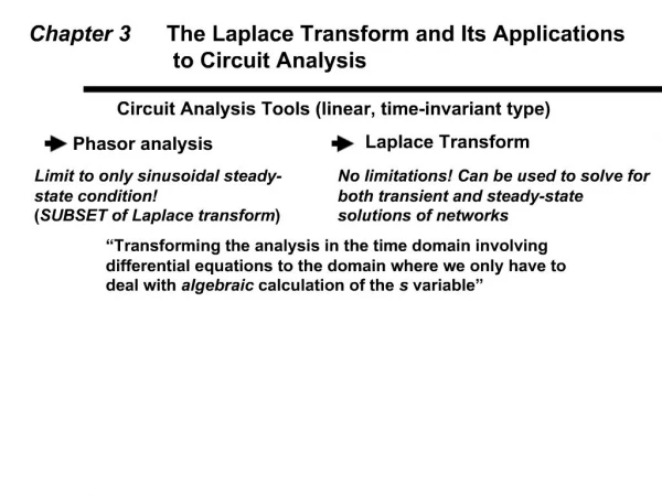
Introduction to Laplace Transform: Key Concepts and Applications
140 likes | 517 Views
Learn the basics of Laplace transform, its relation to Fourier transform, properties, and examples. Understand the region of convergence and how it applies to analyzing signals and stability.

Introduction to Laplace Transform: Key Concepts and Applications
E N D
Presentation Transcript
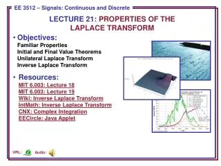
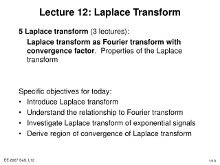
Lecture 12: Laplace Transform • 5 Laplace transform (3 lectures): • Laplace transform as Fourier transform with convergence factor. Properties of the Laplace transform • Specific objectives for today: • Introduce Laplace transform • Understand the relationship to Fourier transform • Investigate Laplace transform of exponential signals • Derive region of convergence of Laplace transform
Lecture 12: Resources • Core material • SaS, O&W, Chapter 9.1&9.2 • Recommended material • MIT, Lecture 17 • Note that in the next 3 lectures, we’re looking at continuous time signals (and systems) only
Introduction to the Laplace Transform • Fourier transforms are extremely useful in the study of many problems of practical importance involving signals and LTI systems. • purely imaginary complex exponentials est, s=jw • A large class of signals can be represented as a linear combination of complex exponentials and complex exponentials are eigenfunctions of LTI systems. • However, the eigenfunction property applies to any complex number s, not just purely imaginary (signals) • This leads to the development of the Laplace transform where s is an arbitrary complex number. • Laplace and z-transforms can be applied to the analysis of un-stable system (signals with infinite energy) and play a role in the analysis of system stability
The Laplace Transform • The response of an LTI system with impulse response h(t) to a complex exponential input, x(t)=est, is • where s is a complex number and • when s is purely imaginary, this is the Fouriertransform, H(jw) • when s is complex, this is the Laplace transform of h(t), H(s) • The Laplace transform of a general signal x(t) is: • and is usually expressed as:
Laplace and Fourier Transform • The Fourier transform is the Laplace transform when s is purely imaginary: • An alternative way of expressing this is when s = s+jw • The Laplace transform is the Fourier transform of the transformed signal x’(t) = x(t)e-st. Depending on whether s is positive/negative this represents a growing/negative signal
Example 1: Laplace Transform • Consider the signal • The Fourier transform X(jw) converges for a>0: • The Laplace transform is: • which is the Fourier Transform of e-(s+a)tu(t) • Or • If a is negative or zero, the Laplace Transform still exists
Example 2: Laplace Transform • Consider the signal • The Laplace transform is: • Convergence requires that Re{s+a}<0 or Re{s}<-a. • The Laplace transform expression is identical to Example 1 (similar but different signals), however the regions of convergence of s are mutually exclusive (non-intersecting). • For a Laplace transform, we need both the expression and the Region Of Convergence (ROC).
Example 3: sin(wt)u(t) • The Laplace transform of the signal x(t) = sin(wt)u(t) is:
Fourier Transform does not Converge … • It is worthwhile reflecting that the Fourier transform does not exist for a fairly wide class of signals, such as the response of an unstable, first order system, the Fourier transform does not exist/converge • E.g. x(t) = eatu(t), a>0 • does not exist (is infinite) because the signal’s energy is infinite • This is because we multiply x(t) by a complex sinusoidal signal which has unit magnitude for all t and integrate for all time. Therefore, as the Dirichlet convergence conditions say, the Fourier transform exists for most signals with finite energy
Im Im -a -a Re Re Region of Convergence • The Region Of Convergence (ROC) of the Laplace transform is the set of values for s (=s+jw) for which the Fourier transform of x(t)e-st converges (exists). • The ROC is generally displayed by drawing separating line/curve in the complex plane, as illustrated below for Examples 1 and 2, respectively. • The shaded regions denote the ROC for the Laplace transform
Example 4: Laplace Transform • Consider a signal that is the sum of two real exponentials: • The Laplace transform is then: • Using Example 1, each expression can be evaluated as: • The ROC associated with these terms are Re{s}>-1 and Re{s}>-2. Therefore, both will converge for Re{s}>-1, and the Laplace transform:
Lecture 12: Summary • The Laplace transform is a superset of the Fourier transform – it is equal to it when s=jw i.e. F{x(t)} = X(jw) • Laplace transform of a continuous time signal is defined by: • And can be imagined as being the Fourier transform of the signal x’(t) = x(t)est, when s=s+jw • The region of convergence (ROC) associated with the Laplace transform defines the region in s (complex) space for which the Laplace transform converges. • In simple cases it corresponds to the values for s (s) for which the transformed signal has finite energy
Questions • Theory • SaS, O&W, Q9.1-9.4, 9.13 • Matlab • There are laplace() and ilaplace() functions in the Matlab symbolic toolbox • >> syms a w t s • >> laplace(exp(a*t)) • >> laplace(sin(w*t)) • >> ilaplace(1/(s-1)) • Try these functions to evaluate the signals of interest • These use the symbolic integration function int()