Download

1 / 11
110 likes | 138 Views
FAUST Oblique Analytics utilize ScalarPTreeSet (SPTS) for linear and dot product-based insights, with algorithms for clustering, density thresholds, and outlier detection. The techniques consider metrics like Standard Deviation (STD), Average-to-Median (AM), and Precipitous Count Change (PCC) to enhance prediction and classification accuracy through Polygon Prediction (FP.2) and Distance Analytics. The guided approach involves selecting optimal DensityThreshold (DT), DensityUniformityThreshold (DUT), and NextD plans for effective partitioning and analysis. The methodologies factor in outlier mining, fuzzy classification, and the Square Distance To Nearest Neighbor (D2NN) for robust analytics and strategic decision-making. FAUST's innovative algorithms emphasize precision, efficiency, and adaptability in predictive analytics.

E N D
FAUST Oblique Analytics are based on a linear or dot product, oLet X(X1...Xn) be a table. FAUST Oblique analytics employ the ScalarPTreeSet (SPTS) of a valueTree, XoD k=1..nXk*Dk, D=(D1...Dn)=a fixed vector. FAUST Count Change (FC2) for clustering Choose a nextD recursion plan to specify which D to use at each recursive step, e.g., if a cluster, C, needs further partitioning, a. D = the diagonal producing the maximum Standard Deviation (STD(C)) or maximum STD(C)/Spread(C). b. AM(C) (Average-to-Median) c. AFFA(C) (Avg-FurthestFromAverage) [or FFAFFF(C) (FurthestFromAvg-FurthestFromFurthest)]. d. cycle thru diagonals: e1,...,..en, e1e2.. Or cycle thru AM, AFFA, FFAFFF or cycle through both. Choose DensityThreshold(DT), DensityUniformityThreshold(DUT),Precipitous Count Change (PCC) def (PCCs include gaps). ALGORITHM: If DT (and DUT) are not exceeded at cluster, C, partition by cutting at each PCC in CoD using the nextD. FAUST Polygon Prediction (FP 2)for 1-class or multi-class classification. Let Xn+1= Class label column, C. For each vector, D, let lD,kminCkoD (or the1stPrecipitous_Count_Increase=PCI?); hD,k=hD,kmaxCkoD (or the last PCD?). ALGORITHM: y is declared to be class=k iffyHullkwhere Hullk={z| lD,k Doz hD,k all D}. (If y is in multiple hulls, Hi1..Hih, y isaCk for the k maximizing OneCount{PCk&PHi..&PHih} or fuzzy classify using those OneCounts as k-weights) Outlier Mining can mean: 1. Given a set of n objects and given a k, find the top k objects in terms of dissimilarity from the rest of the objects. 1.a This could mean the k object, xh, (h=1..k) most dissimilar [distant from] their individual complements, X-{xh}, or 1.b The top "set of k objects“, Sk, for which that set is most dissimilar from its complement, X-Sk. 2. Given a Training Set, identify outliers in each class (correctly classified but noticeably dissimilar to fellow class members). 3. Determine "fuzzy" clusters, i.e., assign a weight for each (object, cluster) pair. (A dendogram does that to some extent.). Note: FC3 is a good outlier detector, since it identifies and removes large clusters so small clusters (outliers) appear. FAUST Distance Analytics use the SPTS of the distance valueTree, SquareDistanceToNearestNeighbor (D2NN) FAUST Outlier Observer (FO2) uses D2NN. (L2 or Euclidean distance is best, but L (EIN) works too.) D2NN provides an instantaneous k-slider for 1.a (Find k objects, x, most dissimilar from X-{x}. It’s useful for the others too. I say “instantaneous” because the Univariate Distribution Revealer on D2NN takes log2n time (one time only), then the slider works instantaneously off the high end of that distribution.
D2,0 D2,0 D2,1 D2,1 D1,0 D1,0 D1,1 D1,1 D D XoD = k=1..nXk*Dk 1 0 1 1 1 2 3 3 0 1 1 1 k=1..n ( = 22B Dk,B pk,B k=1..n ( Dk,B pk,B-1 + Dk,B-1 pk,B + 22B-1 k=1..n ( Dk,B pk,B-2 + Dk,B-1 pk,B-1 + Dk,B-2 pk,B + 22B-2 Xk*Dk = Dkb2bpk,b XoD=k=1,2Xk*Dk with pTrees: qN..q0, N=22B+roof(log2n)+2B+1 k=1..n ( +Dk,B-3 pk,B Dk,B pk,B-3 + Dk,B-1 pk,B-2 + Dk,B-2 pk,B-1 + 22B-3 = Dk(2Bpk,B +..+20pk,0) = (2BDk,B+..+20Dk,0) (2Bpk,B +..+20pk,0) . . . k=1..2 ( = 2BDkpk,B +..+ 20Dkpk,0 = 22 Dk,1 pk,1 k=1..n ( Dk,Bpk,B) = 22B( +Dk,Bpk,B-1) + 22B-1(Dk,B-1pk,B Dk,B pk,0 + Dk,2 pk,1 + Dk,1 pk,2 +Dk,0 pk,3 + 23 +..+20Dk,0pk,0 k=1..2 ( Dk,1 pk,0 + Dk,0 pk,1 + 21 pTrees k=1..n ( X Dk,2 pk,0 + Dk,1 pk,1 + Dk,0 pk,2 + 22 B=1 1 3 2 1 0 1 0 1 1 1 1 0 0 0 0 1 0 1 k=1..2 ( k=1..n ( Dk,0 pk,0 Dk,1 pk,0 + Dk,0 pk,1 + 20 + 21 q0 = p1,0 = no carry 1 1 0 k=1..n ( Dk,0 pk,0 + 20 ( ( = 22 = 22 1 p1,1 D1,1p1,1 + 1 p2,1 ) + D2,1p2,1 ) ( ( ( ( + 1 p2,0 ) + D2,0p2,0) D1,1p1,0 1 p1,0 + D1,0p11 + 1 p11 1 p1,0 D1,0p1,0 + 21 + 21 + D2,1p2,0 + 1 p2,0 + D2,0p2,1) + 1 p2,1 ) + 20 + 20 q1= carry1= 1 1 0 0 0 1 ( = 22 D1,1 p1,1 + D2,1 p2,1 ) ( ( + D2,0 p2,0) D1,1 p1,0 +D1,0 p11 D1,0 p1,0 + 21 + D2,1 p2,0 +D2,0 p2,1) + 20 0 0 0 q2=carry1= no carry 0 1 1 1 0 1 1 1 0 0 0 1 q0 = carry0= 0 1 1 1 0 0 0 1 1 0 1 1 1 1 0 0 0 0 1 1 0 1 0 1 1 0 1 1 1 1 2 1 1 q1=carry0+raw1= carry1= 1 1 1 1 1 1 q2=carry1+raw2= carry2= 1 1 1 q3=carry2 = carry3= A carryTree is a valueTree or vTree, as is the rawTree at each level (rawTree = valueTree before carry is incl.). In what form is it best to carry the carryTree over? (for speediest of processing?) 1. multiple pTrees added at next level? (since the pTrees at the next level are in that form and need to be added) 2. carryTree as a SPTS, s1? (next level rawTree=SPTS, s2, then s10& s20 = qnext_level and carrynext_level ? FLC ClustererChoose nextD plan, a Density (DT) and a DensUnif(DUT) threshold and a PrecipCountChange (PCC) Def. If DT (and/or DUT) are not exceeded at C, partition C further by cutting at each gap and PCC in CoD using the nextD. For a table X(X1...Xn), the SPTS, Xk*Dk is the column of numbers, xk*Dk. XoD is the sum of those SPTSs, k=1..nXk*Dk
FDO D2NN(x): (x-X)o(x-X) = k=1..n(xk-Xk)(xk-Xk)=k=1..n(b=B..02bxk,b-2bpk,b)( (b=B..02bxk,b-2bpk,b) Table, X(X1...Xn) D2NN yields a 1.a-type outlier detector (top k objects, x, dissimilarity from X-{x}). pTrees X We install in D2NN, each min[D2NN(x)] (It's a one-time construction but for a trillion x's it will take a while. Is there a massive parallelization scheme?) 1 3 2 1 0 1 0 1 1 1 1 0 0 0 0 1 0 1 =k=1..n( b=B..02b(xk,b-pk,b) )( b=B..02b(xk,b-pk,b) ) |---ak,b---| = k=1..n =k=1..n( b=B..0 2bak,b ) ( b=B..0 2bak,b ) ( 2Bak,B + 2B-1ak,B-1 +...+ 21ak, 1 + 20ak, 0 ) ( 2Bak,B + 2B-1ak,B-1 +...+ 21ak, 1 + 20ak, 0 ) ( 22Bak,Bak,B + 22B-1( ak,Bak,B-1 + ak,B-1ak,B ) + { which is 22Bak,Bak,B-1 } 22B-2( ak,Bak,B-2 + ak,B-1ak,B-1 + ak,B-2ak,B ) + { which is 22B-1ak,Bak,B-2 + 22B-2ak,B-12 22B-3( ak,Bak,B-3 + ak,B-1ak,B-2 + ak,B-2ak,B-1 + ak,B-3ak,B ) + { 22B-2( ak,Bak,B-3 + ak,B-1ak,B-2 ) } 22B-4(ak,Bak,B-4+ak,B-1ak,B-3+ak,B-2ak,B-2+ak,B-3ak,B-1+ak,B-4ak,B)+ {22B-3( ak,Bak,B-4+ak,B-1ak,B-3)+22B-4ak,B-22} {h odd: 22B-h+1i=B..B-(h-1)/2ak,iak,2B-h-i {h even 22B-h+1i=B..B+1-h/2ak,iak,2B-h-i +22B-hak,B-h/22 22B-h(ak,Bak,B-h+ak,B-1ak,B-h+1+...+ak,B-h+1ak,B-1+ak,B-hak,B)
FDO D2NN(x)= k=1..n(xk-Xk)(xk-Xk)=k=1..n(b=B..02bxk,b-2bpk,b)( (b=B..02bxk,b-2bpk,b) ----ak,h-- b=B..02b(xk,b-pk,b) ) =k=1..n( b=B..02b(xk,b-pk,b) )( =k =k=1..n(b=B..02bak,b)( b=B..02bak,b) (2Bak,B+ 2B-1ak,B-1+..+ 21ak, 1+ 20ak, 0) (2Bak,B+ 2B-1ak,B-1+..+ 21ak, 1+ 20ak, 0) Table, X(X1...Xn) D2NN yields a 1.a-type outlier detector (top k objects, x, dissimilarity from X-{x}). We install in D2NN, each min[D2NN(x)] (It's a one-time construction but for a trillion x's it;s slow. Parallelization?) pTrees X 1 3 2 1 0 1 0 1 1 1 1 0 0 0 0 1 0 1 ( 22Bak,Bak,B + 22B-1( ak,Bak,B-1 + ak,B-1ak,B ) + { which is 22Bak,Bak,B-1 } 22B-2( ak,Bak,B-2 + ak,B-1ak,B-1 + ak,B-2ak,B ) + { which is 22B-1ak,Bak,B-2 + 22B-2ak,B-12 22B-3( ak,Bak,B-3 + ak,B-1ak,B-2 + ak,B-2ak,B-1 + ak,B-3ak,B ) + { 22B-2( ak,Bak,B-3 + ak,B-1ak,B-2 ) } 22B-4(ak,Bak,B-4+ak,B-1ak,B-3+ak,B-2ak,B-2+ak,B-3ak,B-1+ak,B-4ak,B)... {22B-3( ak,Bak,B-4+ak,B-1ak,B-3)+22B-4ak,B-22} 22B ( ak,B2 + ak,Bak,B-1 ) + 22B-1( ak,Bak,B-2 ) + 22B-2( ak,B-12 + ak,Bak,B-3 + ak,B-1ak,B-2 ) 22B-3( ak,Bak,B-4+ak,B-1ak,B-3) 22B-4ak,B-22 ...
FLC on IRIS150 DT=1 PCCD: PCCs must involve a hi 5 and be at least a 60% change ( 2 if high=5) from that high. Gaps must be 3 FLC on IRIS150: 1st rnd, D=1-111(hi STD/spread = 28.2 and high Spread=121) 91.3% accurate after 1st round F 0 1 2 3 4 5 6 7 8 9 22 23 24 26 27 28 29 30 31 32 33 34 35 36 37 38 39 40 41 42 43 45 46 47 48 49 50 51 52 53 54 55 57 60 Ct 1 1 2 3 7 14 12 4 5 1 2 1 1 1 2 2 4 5 5 6 2 3 5 2 3 5 6 6 5 2 6 5 4 4 3 1 1 2 1 1 1 1 1 1 Gp 1 1 1 1 1 1 1 1 1 13 1 1 2 1 1 1 1 1 1 1 1 1 1 1 1 1 1 1 1 1 2 1 1 1 1 1 1 1 1 1 1 2 3 ----------------(50 0 0)-------- C1(0 25 2) (090) C2(0 16 11) (0 0 37) 2nd rnd, D=1-1-1-1 (which is the highest STD/spread of those to 1-111: 111-1 11-11 1-1-1-1) C2 14 15 16 17 19 21 22 23 24 25 26 28 29 31 32 33 35 38 1 1 3 2 1 1 1 1 2 1 1 1 3 1 1 4 1 1 1 1 1 2 2 1 1 1 1 1 2 1 2 1 1 2 3 C21(0 3 10) (021) ----(0 11 0)----- C1 F 17 19 21 27 28 29 30 32 33 34 35 36 37 39 40 41 49 Ct 1 1 1 3 3 1 1 1 1 1 4 1 2 2 2 1 1 Gp 2 2 6 1 1 1 2 1 1 1 1 1 2 1 1 8 (001) (020) (0 23 0) (001) 97.3% accurate after 2nd round For big datasets, gaps will not appear, so we will have to rely on PCCs only. Next I look at IRIS using only PCCs and hope to find that it doesn't matter what D we pick in that case except for speed and cleanliness. FLC on IRIS150: 1st rnd, D=1-111 F 0 1 2 3 4 5 6 7 8 9 22 23 24 26 27 28 29 30 31 32 33 34 35 36 37 38 39 40 41 42 43 45 46 47 48 49 50 51 52 53 54 55 57 60 Ct 1 1 2 3 7 14 12 4 5 1 2 1 1 1 2 2 4 5 5 6 2 3 5 2 3 5 6 6 5 2 6 5 4 4 3 1 1 2 1 1 1 1 1 1 ----------------(49 0 0)----- C1(1 25 2) (090) C2(0 16 11) (0 0 37) 1strnd: 14 errs FLC on IRIS150: 1st rnd, D=0001 (14 0 0) F 0 1 2 3 4 5 9 10 11 12 13 14 15 16 17 18 19 20 21 22 23 24 Ct 6 28 7 7 1 1 7 3 5 13 8 12 4 2 12 5 6 6 3 8 3 3 (600)(2800) (200) (070)(080)(0 30 3) (042) (0 1 31) (0 0 14) 1strnd: 6 errs (highest STD.Spread=0,31 tied with 3+4. FLC on IRIS150: 1st rnd, D=0010 1strnd: 52 errs (STD.Spread=0.29 F 0 1 2 3 4 5 6 7 8 9 20 23 25 26 27 28 29 30 31 32 33 34 35 36 37 38 39 40 41 42 43 44 45 46 47 48 49 50 51 53 54 56 57 59 Ct 1 1 2 7 12 14 7 4 1 2 1 2 2 1 1 1 3 5 3 4 2 4 8 3 5 3 5 4 8 2 2 2 3 6 3 3 2 2 3 1 1 1 2 1 (400) (46 36 2) (0 14 14) (0 0 24) NOTE: [3,8)=(44 0 0) [8,36)=(2 36 2) [36,38)=(080)
FLC on SEED150DT=1 PCCs have to involve a high of at least 5 and be at least 60% change from that high. Gaps must be 3 NSTD 1 2 3 4 0.28 0.28 0.22 0.47 NSTD Std(Xk-minXk)/SpreadXk ? C2 (1L, 0M, 0H) 2nd round D=AFFA 22 25 27 29 31 33 34 35 37 39 42 43 44 45 46 48 49 50 51 52 53 54 55 1 1 2 6 4 1 1 2 3 3 1 1 1 5 4 7 1 3 2 5 1 3 3 3 2 2 2 2 1 1 2 2 3 1 1 1 1 2 1 1 1 1 1 1 1 1 56 57 58 59 60 61 62 63 64 65 68 69 70 71 72 4 3 4 1 3 1 13 1 10 6 3 2 7 1 2 1 1 1 1 1 1 1 1 1 3 1 1 1 1 C1,3,2 (0L,1M,0H) C1,3,3 (0L,0M,2H) The Ulitmate PCC clusterer algorithm ? Set Dk to 1 for each column with NSTD>ThresholdNSTD (NSTDT=0.25) Shift X column values as in Gap Preservation above giving the shifted table, Y Make Gap and PCC cuts on YoD If Density < DT at a dendogram node, C, (a cluster), partition C at each gap and PCC in CoD using next D in recursion plan. Using UPCC with D=1111 First round only: F 0 1 2 3 4 5 6 7 8 9 10 11 12 13 14 15 16 17 Ct 1 6 10 22 25 16 12 1 9 6 14 12 7 3 1 3 1 1 GP 1 1 1 1 1 1 1 1 1 1 1 1 1 1 1 1 1 C1 (44L, 1M, 47H) C4 (2L, 31M, 0H) C5 (0L, 9M, 0H) C3 (3L, 9M, 3H) errs=53 45 0 6 2 0 spread=10 3 1 3 2 1 Using UPCC with D=1001 First round only: F 0 1 2 3 4 5 6 7 8 9 10 11 Ct 18 25 18 18 14 6 9 7 8 21 2 4 GP 1 1 1 1 1 1 1 1 1 1 1 C2 (0L, 22M, 0H) C3 (8L, 21M, 0H) C1 (42L, 1M, 50H) C4 (0L, 6M, 0H) errs=51 43 0 8 0 spread=6 2 1 2 1 (0L,0M,1H) C1.5.5 (0L,0M,1H) C1.4.5 D=1101 1st rnd: 85% accurate 0 1 2 3 4 5 6 7 8 9 10 11 12 13 18 25 16 9 13 12 6 9 7 7 21 1 3 3 1 1 1 1 1 1 1 1 1 1 1 1 1 C1,1 (0L,4M,0H) C1,8 (3L,0M,28H) C1,2 (6L,17M,0H) C1,3 (13L,1M,2H) C1,5 (5L,0M,0H) C1,6 (16L,0M,6H) C1,7 (2L,0M,12H) C3 (0L,7M, 0H) C1,4 (5L,0M,0H) C1 (50L,22M,50H) C2 (0L,21M,0H) 3rd round D=0010 C1,6: 3rd round D=0010 C1,8: C1,2 3rdrnd D=0010 errs=72 72 0 0 spread=5 3 1 1 F 0 1 Ct 4 19 GP 1 F 0 1 2 3 4 5 6 7 Ct 2 5 6 5 1 1 1 1 F 0 1 2 3 4 5 Ct 3 2 2 17 3 4 C1,2,1 (4L,0M,0H) C1,2,1 (2L,17M) C1,6,2 (14L,0M,2H) C1,8,1 (3L,0M,0H) C1,6,1 (2L,0M,0H) C1,6,3 (0L,0M,4H) C1,8,2 (0L,0M,28H) 3rd round D=0010 C1,3: 3rd round with D=0010 97.3% accurate F 0 1 2 3 6 7 Ct 3 5 4 1 1 2 C1,3,1 (3L,0M,0H) C1,3,2 (9L,0M,0H)
FLC on CONC150 CONC counts are L=43, M=52, H=55 DT=1PCCs: 5 60% change from high. Gaps: 3 NSTD 1 2 3 4 0.25 0.25 0.24 0.22 COLUMN 1 2 3 4 STD .017 .005 .001 .037 SPREAD 10 39 112 5.6 STD/SPR .18 .23 .21 2.38 NSTD Std(Xk-minXk)/SpreadXk ? NSTD Std(Xk-minXk)/SpreadXk ? (1 0 0) C3(14 17 1) C5(1 20 4) (0 0 2) F 0 1 2 3 4 5 6 Ct 1 27 32 53 25 10 2 C2(22 4 1) C4(18 28 7) C6(1 6 3) D 0001 1st rnd Gp>=1 0 1 6 7 8 10 14 15 16 17 18 20 21 22 23 24 25 26 28 29 31 33 34 36 1 1 1 1 1 1 1 2 1 1 2 2 2 2 1 2 2 4 1 3 1 1 2 1 1 5 1 1 2 4 1 1 1 1 2 1 1 1 1 1 1 2 1 2 2 1 2 1 (200) C2(2,2,0) 37 38 39 40 41 42 43 44 45 46 48 49 50 51 52 53 54 55 56 58 59 61 62 1 2 1 1 2 1 2 1 5 4 2 6 1 1 4 1 1 7 1 3 2 1 5 1 1 1 1 1 1 1 1 1 2 1 1 1 1 1 1 1 1 2 1 2 1 1 C3(24 13 5) C4(6,4,1)(204) C6(5,6,11) C5 D 1111 1st rnd 1st rnd 53% accurate 63 64 65 66 67 68 69 71 72 73 74 76 77 78 80 81 82 85 86 87 91 92 94 3 3 1 2 1 2 1 1 2 1 1 1 1 1 1 5 3 5 2 2 5 1 1 1 1 1 1 1 1 2 1 1 1 2 1 1 2 1 1 3 1 1 4 1 2 3 C9(0 11 16) C10(152)(005)C11(144) (002) 97 98 100 101 102 104 110 119 F 1 3 2 2 1 1 1 1 Count 1 2 1 1 2 6 9 Gap C15(0 5 5) (0 2 0) (030) F 51 57 58 63 64 83 Ct 1 1 3 1 1 1 GP 6 1 5 1 19 (100)(001) (011) (010) F 71 74 119 Ct 1 1 4 GP 3 45 (200) (004) (100) (100) (0 0 9) (010) F 8 16 24 27 28 29 37 41 42 45 48 49 51 67 73 Ct 1 1 1 2 2 1 1 1 1 1 4 2 2 1 1 GP 8 8 3 1 1 8 4 1 3 3 1 2 16 6 (020) ( 2 2 1) (110) (001) F 31 37 41 49 Ct 1 1 1 1 GP 6 4 8 (200) (020) (010) F 20 42 58 64 77 83 Ct 1 2 3 1 2 1 GP 22 16 6 13 6 (010)(0 0 5) (0 4 0) (310) (610) (002) (102) (1 2 0) F 21 26 31 32 36 51 53 64 68 71 100 102 109 112 121 122 Ct 2 3 4 3 1 4 3 2 7 2 2 2 3 1 1 2 GP 5 5 1 4 15 2 11 4 3 29 2 7 3 9 1 (5 0 0)(520)(100) (0 5 0) (101) (020) (100) (010) (002) (011) F 16 20 24 29 37 48 49 51 52 54 57 63 64 67 73 82 83 Ct 1 1 1 1 2 4 1 1 3 1 3 1 1 2 2 1 1 GP 4 4 5 8 11 1 2 1 2 3 6 1 3 6 9 1 (0 4 0) (002) (0 2 8) (012)(020) (011) D:1100 2nd rnd C9 (0 11 16) D:1100 2nd rnd C15 (0 5 5) D:1100 2nd rn10 C10 (1 5 2) D:1100 2nd rnd C6 (56 11) D:1100 2nd rnd C3 (24 13 5) D:1100 2nd rnd C2 (22 0) D:1100 2nd rnd C5 (2 0 4) (200) F 14 16 24 28 48 49 51 64 Ct 1 1 2 2 2 1 1 1 GP 2 8 4 20 1 2 13 (200) (101) (140) D:1100 2nd rnd C4 (6 41) (010) (001) F 8 42 54 58 63 73 Ct 1 2 1 3 1 1 GP 34 12 4 5 10 (010)(110) (003) (010) D:1100 2nd rn10 C11 (1 4 4) FLC on WINE150 WINE counts are L=57, M=75, H=18 DT=1 PCCs: 5 60% change from high. 2nd round 90% accurate 1st round 64% accurate F 1 2 3 4 6 7 8 9 10 11 13 14 17 19 23 24 29 Ct 2 1 2 1 3 3 3 2 1 2 1 1 1 1 1 1 1 GP 1 1 1 2 1 1 1 1 1 2 1 3 2 4 1 5 C21(5 0 1) C22(10 4 0) (7 0 0) (030) F 0 2 3 4 5 6 7 8 9 10 11 12 13 17 18 20 21 22 24 25 27 32 37 Ct 1 3 4 2 3 2 4 1 2 1 1 2 2 4 1 2 2 3 2 1 1 1 2 GP 2 1 1 1 1 1 1 1 1 1 1 1 4 1 2 1 1 2 1 2 5 5 3 C31(10 8 1) C32(1 5 3) C33(121) C34(4 7 1) C35(481) C2 0100 2nd rnd (22 4 1) Gp>=2 C4 0010 2nd rnd (18 28 7) (020) (010) 40 52 60 67 93 106 1 1 1 1 1 1 12 8 7 26 13 (100) (001) (100) F 10 12 18 20 35 58 79 81 82 Ct 1 1 1 1 1 1 1 2 1 GP 2 6 2 15 23 21 2 1 (002) (030) (100) (031) C6 0010 2nd rnd (18 28 7)
Class1=C1={y1,y2.y3,y4. FLP on IRIS150 C e1 13 12 11 10 e2 23 22 21 20 y1 1 0 0 0 1 1 0 0 0 1 y2 3 0 0 1 1 1 0 0 0 1 y3 2 0 0 1 0 2 0 0 1 0 y4 3 0 0 1 1 3 0 0 1 1 y7 15 1 1 1 1 1 0 0 0 1 y8 14 1 1 1 0 2 0 0 1 0 y9 15 1 1 1 1 3 0 0 1 1 yb 10 1 0 1 0 9 1 0 0 1 yc 11 1 0 1 1 10 1 0 1 0 yd 9 1 0 0 1 11 1 0 1 1 ye 11 1 0 1 1 11 1 0 1 1 mn1 1 mx1 3 mn2 1 mx2 3 mn1+2 2 mx1+2 6 mn1-2 0 mx1-2 2 mn1 14 mx1 15 mn2 1 mx2 3 mn1+2 16 mx1+2 18 mn1-2 12 mx1-2 14 mn1 9 mx1 11 mn2 9 mx2 11 mn1+2 20 mx1+2 22 mn1-2 -1 mx1-2 1 Class2=C2={y7,y8.y9}. Class3=C3={yb,yc.yd,ye} Shortcuts ? Pre-compute all diagonal mins and maxs; e1, e2, e1+e2, e1-e2. Then there is no pTree processing left to do (just straight forward comparisons). xCk iff lok,D Dox hik,D D. 1 y1y2y7 2 y3y5 y8 y 3 y4 y6 y9 4 ya 5 6 7 8 yf 9 yb ax yc b yd ye 0 1 2 3 4 5 6 7 8 9 a b c d e f xf 7 One1 it is "none-or-the-above" 9,a 9 -1 1910 It is in class3 (red) only ya13 On e1 it is "none-or-the-above" y5 5 2 On e1 it is "none-or-the-above" f,215 13 172 It is in class2 (green) only Versicolor 1D min 49 20 33 10 max 70 34 51 18 n1 n2 n3 n4 x1 x2 x3 x4 1D FLP Hversicolor has 7 virginica! Versicolor 2D min 70 82 59 55 59 43 24 9 38 -24 7 23 max 102 118 84 80 84 67 40 23 56 -7 18 35 n12 n13 n14 n23 n24 n34 n1-2 n1-3 n1-4 n2-3 n2-4 n3-4 x12 x13 x14 x23 x24 x34 x1-2 x1-3 x1-4 x2-3 x2-4 x3-4 1D_2D FLP Hversicolor has 3 virginica! 1D_2D_3D FLP Hversicolor has 3 virginica! Versicolor 3D min 105 80 92 65 35 58 -21 60 35 max 149 116 134 98 55 88 -2 88 55 n123 n124 n134 n234 n12-3 n1-23 n1-2-3 n12-4 n1-24 x123 x124 x134 x234 x12-3 x1-23 x1-2-3 x12-4 x1-24 9 72 24 -7 45 -9 -40 28 103 37 12 65 6 -19 n1-2-4 n13-4 n1-34 n1-3-4 n23-4 n2-34 n2-3-4 x1-2-4 x13-4 x1-34 x1-3-4 x23-4 x2-34 x2-3-4 Versicolor 4D min 115 95 45 68 20 48 -6 -39 max 164 135 69 104 41 74 10 -12 n1234 n123-4 n12-34 n1-234 n12-3-4 n1-23-4 n1-2-34 n1-2-3-4 x1234 x123-4 x12-34 x1-234 x12-3-4 x1-23-4 x1-2-34 x1-2-3-4 1D_2D_3D_4D MCL Hversicolor has 3 virginica (24,27,28) 1D_2D_3D_4D FLP Hvirginica has 20 versicolor errors!! Look at removing outliers (gapped>=3) from Hullvirginica 23 Ct gp 48 1 22 70 1 2 72 1 3 75 2 1 ''' 96 1 1 97 1 5 102 1 3 105 1 e1 Ct gp 49 1 7 56 1 1 ... 77 4 2 79 1 e2 Ct gp 22 1 3 25 4 1 ... 36 1 2 38 2 e3 Ct gp 18 1 27 45 1 3 ... 67 2 2 69 1 e4 Ct gp 14 1 1 24 3 1 25 3 12 Ct gp 74 1 8 82 2 2 ... 117 1 13 Ct gp 78 1 16 94 1 10 104 ... 146 14 Ct gp 66 1 9 75 2 1 ... 102 1 24 Ct gp no outliers 34 Ct gp 36 1 26 62 1 3 65 1 1 ... 89 1 3 92 1 Hvirginica 12 versic Hvirginica 3 versic Hvirginica 15 versic 1D FLP Hvirginica only 16 versicolors! One possibility would be to keep track of those that are outliers to their class but are not in any other class hull and put a sphere around them. Then any unclassified sample that doesn't fall in any class hull would be checked to see if it falls in any of the class outlier spheres???
1 y1y2 y7 2 y3 y5 y8 3 y4 y6 y9 4 ya 5 6 7 8 yf 9 yb a yc b yd ye 0 1 2 3 4 5 6 7 8 9 a b c d e f 1 y1y2 y7 2 y3 y5 y8 3 y4 y6 y9 4 ya 5 6 7 8 yf 9 yb a yc b yd ye 0 1 2 3 4 5 6 7 8 9 a b c d e f DensityCount/r2 labeled dendogram for FAUST on Spaeth with D=AvgMedian DET=.3 So intersect thinnings [1,1]1, [5,7]1 and [13,14]1 with [4,10]2 1 2 2 1 1 2 1 2 1 1 2 A1 1 2 3 5 7 9 10 11 13 14 15 3 3 3 1 1 1 1 2 A2 1 2 3 4 8 9 10 11 FLC for outlier detectionWhen the goal is to only to find outliers as quickly as possible. 1 recursively uses a vector, D=FurthestFromMedian-to-FurthestFromFurthestFromMedia. Mean=(8.53, 4,73) Median=(9, 3) d2(y1,x), D=y1->y9 0 4 2 8 17 68 196 170 200 153 145 181 164 200 85 xoD = xo(14,2) 16 44 32 48 74 132 212 200 216 190 158 174 148 176 114 FDO-1 won't work for big data. Finding outliers is local. Big data has many localities to exhaustively search. We may need to enclose each outlier in a gapped hulls. Those gapped hulls will likely be filled in when projecting onto a randomly chosen line. I.e., barrel gapping suffers from a chicken-egg problem: First look for linear gaps and then radial gaps out from it. Unless line runs thru outlier radial gap not likely to appear xoD2 13. 14. 12. 11. 13. 13. 20. 17. 16. 14 3.9 2.6 0 0.9 4.2 xoD3 1.6 4.3 3.3 5 7.3 13 20. 19. 21 18. 16. 18 15. 18. 12 d2(med,x) 68 40 50 36 17 0 40 26 36 17 37 53 64 68 29 y1 y2 y3 y4 y5 y6 y7 y8 y9 ya yb yc yd ye yf xoD Distribution down to 25: 1 3 1 1 3 3 3 [0,32) [32,64) [64,96) [96,128) [128,160) [160,192) [192,224) Thinnings [0,32) and [64,128). So we check y1,y5,yf. y5 and yf check out as outliers, y1 does not. Note y6 does not either! Let D2 be mean to median and go down to 22: 0 1 1 6 2 1 [0,4) [4,8) [8,12) [12,16) [16,20) [20,24) Thinnings [4,12), [20,24). yf checks out as outlier, y4 does not. Note y6 does not either! Let D3 be (Median to FurthestFromMedian)/6 and go down to 22: 2 3 1 2 5 2 [0,4) [4,8) [8,12) [12,16) [16,20) [20,24) Thinnings [8,16) yf , y6 check out as outlier, yd does not. This D3 isd best? FOD-1 doesn't work well for interior outlier identifiction (which is the case for all Spaeth outliers. 2uses FLC Clusterer (CC=Count Change) to find outliers. CC removes big clusters so that as it moves down the dendogram clusters gets smaller and smaller. Thus outliers are more likely to reveal themselves as singletons (and doubletons?) gapped away from their complements. With each dendogram iteration we will attempt to identify outlier candidates and construct the SPTS of distances from each candidate (If the minimum of those distance exceeds a threshold, declare that candidate an outlier.). E;g;, look for outliers using projections onto the sequence of D's = e1,...,en , then diagonals, e1+e2, e1-e2, ... We look for singleton (and doubleton?...) sets gapped away from the other points. We start out looking for coordinate hulls (rectangles) that provide a gap around 1 (or2? or 3?) points only. We can do this by intersecting "thinnings" in each DoX distribution. ote, if all we're interested in anomalies, then we might ignore all PCCs that are not involved in thinnings. This would save lots of time! (A "thinning" is a PCD to below threshold s.t. the next PCC is a PCI to above threshold. The threshold should be PCC threshold.)
pTrees XoD = k=1..nXk*Dk k=1..n ( = 22B Dk,B pk,B k=1..n ( Dk,B pk,B-1 + Dk,B-1 pk,B + 22B-1 k=1..n ( Dk,B pk,B-2 + Dk,B-1 pk,B-1 + Dk,B-2 pk,B + 22B-2 k=1..n ( Dk,B pk,B-3 + Dk,B-1 pk,B-2 + Dk,B-2 pk,B-1 +Dk,B-3 pk,B + 22B-3 . . . k=1..n ( Dk,B pk,0 + Dk,2 pk,1 + Dk,1 pk,2 +Dk,0 pk,3 + 23 k=1..n ( Dk,2 pk,0 + Dk,1 pk,1 + Dk,0 pk,2 + 22 k=1..n ( Dk,1 pk,0 + Dk,0 pk,1 + 21 k=1..n ( Dk,0 pk,0 + 20 X Appendix (scratch work) B=1 1 3 2 1 0 1 0 1 1 1 1 0 0 0 0 1 0 1 D2,0 D2,1 D1,0 D1,1 D 1 0 1 2 0 1 XoD=k=1,2Xk*Dk with pTrees: qN..q0, N=22B+roof(log2n)+2B+1 k=1..2 ( = 22 Dk,1 pk,1 k=1..2 ( Dk,1 pk,0 + Dk,0 pk,1 + 21 k=1..2 ( Dk,0 pk,0 + 20 ( = 22 D1,1p1,1 + D2,1p2,1 ) ( ( + D2,0p2,0) D1,1p1,0 + D1,0p11 D1,0p1,0 + 21 + D2,1p2,0 + D2,0p2,1) + 20 ( = 22 D1,1 p1,1 +D2,1 p2,1 ) ( ( + D2,0 p2,0) D1,1 p1,0 +D1,0 p11 D1,0 p1,0 + 21 + D2,1 p2,0 +D2,0 p2,1) + 20 0 0 0 0 1 1 1 0 1 1 1 0 q0=p1,0= no carry q1= carry1= q2=carry1+p2,1= no carry 0 0 1 0 0 1 1 1 0 1 1 0 XoD=k=1,2Xk*Dk with pTrees: qN..q0, N=22B+roof(log2n)+2B+1 Where does this exponent come from? Since x = ( x1,B2B +..+ x1,020 , . . . , xn,B2B+..+ xn,020 ) and D = ( D1,B2B +..+ D1,020 , . . . , Dn,B2B+..+ Dn,020 ) xoD = (x1,B2B +..+ x1,020) (D1,B2B +..+ D1,020) + . . . + (xn,B2B +..+ xn,020) (Dn,B2B +..+ Dn,020)
Xk*Dk = Dkb2bpk,b = Dk(2Bpk,B +..+20pk,0) = (2BDk,B+..+20Dk,0) (2Bpk,B +..+20pk,0) = k=1..n, b=B..0 2bDk pk,b XoD = k=1..nXk*Dk = 2BDkpk,B +..+ 20Dkpk,0 = k=1..n, b=B..0 2b pk,b (2BDk,B+..+20Dk,0) = k=1..n, b=B..0, =B..0 2b+ Dk, pk,b FAUST LINEAR CC ClustererChoose nextD plan, Dens (DT) DensUnif(DUT) thresholds, PrecipCountChange (PCC) If DT (and/or DUT) are not exceeded at C, partition C by cutting at each gap and PCC in CoD using the nextD. Given a table, X(X1...Xn), Xk*Dk is the SPTS (column of numbers) xk*Dk and XoD is the sum of those SPTSs, k=1..nXk*Dk XkDk= 22B ( Dk,B pk,B Dk,B pk,B-1 + Dk,B-1 pk,B + 22B-1 ( Dk,B pk,B-2 + Dk,B-1 pk,B-1 + Dk,B-2 pk,B + 22B-2 ( Dk,B pk,B-3 + Dk,B-1 pk,B-2 + Dk,B-2 pk,B-1 + Dk,B-3 pk,B + 22B-3 ( . . . 0 1 2 . . . . . . . B-1 B = Dk,B pk,0 + Dk,2 pk,1 + Dk,1 pk,2 + Dk,0 pk,3 + 23 ( Dk,2 pk,0 + Dk,1 pk,1 + Dk,0 pk,2 + 22 ( Dk,1 pk,0 + Dk,0 pk,1 + 21 ( Dk,0 pk,0 + 20 ( 0 1 2 B =b XoD = k=1..nXk*Dk k=1..n ( = 22B Dk,B pk,B k=1..n ( Dk,B pk,B-1 + Dk,B-1 pk,B + 22B-1 k=1..n ( Dk,B pk,B-2 + Dk,B-1 pk,B-1 + Dk,B-2 pk,B + 22B-2 k=1..n ( Dk,B pk,B-3 + Dk,B-1 pk,B-2 + Dk,B-2 pk,B-1 + Dk,B-3 pk,B + 22B-3 . . . k=1..n ( Dk,B pk,0 + Dk,2 pk,1 + Dk,1 pk,2 + Dk,0 pk,3 + 23 k=1..n ( Dk,2 pk,0 + Dk,1 pk,1 + Dk,0 pk,2 + 22 k=1..n ( Dk,1 pk,0 + Dk,0 pk,1 + 21 k=1..n ( Dk,0 pk,0 + 20