Download
1 / 54
540 likes | 667 Views
Engr/Math/Physics 25. Chp9: ODE Solns By MATLAB. Bruce Mayer, PE Licensed Electrical & Mechanical Engineer BMayer@ChabotCollege.edu. Learning Goals. Use MATLAB’s ODE Solvers to find Solutions to Ordinary Differential Eqns

E N D
Engr/Math/Physics 25 Chp9: ODE SolnsBy MATLAB Bruce Mayer, PE Licensed Electrical & Mechanical EngineerBMayer@ChabotCollege.edu
Learning Goals • Use MATLAB’s ODE Solvers to find Solutions to Ordinary Differential Eqns • When Possible use Analytical ODE Solutions to Check the ACCURACY of the MATLAB Numerical Soln • Make Approximations to perform a REALITY CHECK on MATLAB Solutions to NONLinear ODEs
MATLAB ODE Solvers • MATLAB has several 1st Order ODE Solver Commands: • ode23 • ode45 (Best OverAll) • ode113 • These Solvers are based on the Runge-Kutta method, which is usually the best technique to apply as a “first try” for most problems.
MATLAB ODE Format - 1 • MATLAB ODE Solver Form for Multiple Dependent Variables (MultiVar Probs) m-Eqns (1st order ODEs) in m-Unknowns
MATLAB Solution • To solve this MultiODE system using MATLAB the functions f1, f2, …, fm must be provided to the computer, along with the initial values of the variables; i.e., t0 and b1,b2, …, bm • The functions f1, f2, …, fm are input using a function which we have to name, say fcn_vec. Then stored in an m-file called in this case fcn_vec.m • The initial values of the y’s are stored in a one dimensional COLUMN vector, say y0
MATLAB Syntax • Obtain the Solution by typing in the command window: [t,y]=ode45(@fcn_vec,Trng,y0) • Where Trng is a vector containing the initial and final values for t. • Example: Trng = [T0 Tf] • Where T0 is set to be t0 and Tf is set to be the final time at the end of the interval of interest.
Plotting the Solution • MATLAB can also be used to plot the ODE Solution results. • For example: plot(t,y) gives a plot of ALL components of the solution y1, y2, …, ym , as a function of t • Alternatively plot(t,y(:,1))gives a plot of y1 as a function of t
Comments on ode45 • Note that in its simplest form ode45 chooses its OWN time step, Δt, and VARIES the time step according to how fast the solution is changing (the steepness of the slope) . • Thus ode45 generates solution values at a sequence of times t1, t2, t3, … given by tk+1= tk+Δtk, with Δtk selected by ode45. • Thus EACH component of the solution y1, y2, …, yn is ITSELF a vector containing values such as y1(t1), y1(t2), y1(t3), …, then y2(t1), y2(t2), y2(t3), …, then y3(t1), y3(t2), y3(t3), etc.
Solve 2ndORDER ODE Example ode45 (1) • Note that to solve a 2nd order eqn we need to know the SLOPE (dy/dt) at t = 0 • To use the 1st Order Solver, cast this 2nd Order eqn into 1st order (state Var) formLET: • With ICs • i.e.,
With the Xform Example ode45 (2) • Subbing in the x1 & x2 • Thus the 1stOrder Eqn System in 2 Vars • Find that • ReArranging the ODE to isolate Highest order term
Note that applying this Xform Example ode45 (3) • And also dx2/dt • Converted the SINGLE 2ndOrder ODE to a LINEAR System of TWO 1stOrder ODEs • Sub into ODE
Now Isolate dx1/dt Example ode45 (4) • Next Isolate dx2/dt • Recall the IC’s
Example ode45 (5) • Thus the Transformation to State-Var Form of Two 1stOrder ODEs • The final xForm
Example ode45 (6) • Compare xForm to Slide-4
The Function File = xdot_lec24.m Example ode45 (7) functionxd = xdot_lec24(t_val,y_vals); % Bruce Mayer, PE * 05Nov11 % ENGR25 * Lec24 on MATLAB ODE solvers % %This is the function that makes up the system %of differential equations solved by ode45 % % the Vector y_vals contains yk & [dy/dt]k % % DEBUG Section %Ttest = t_val; y_vals_test = y_vals; xd % xd(1)=y_vals(2); % at t=0, xdot(1) = dy(0)/dt xd(2)= sin(t_val) -5*y_vals(1) - 2*y_vals(2); % at t=0, xdot(2) = d2y(0)/dt2 % % Must return a COLUMN Vector xd = [xd(1); xd(2)]; % % DEBUG Section disp('xd(1) = dy/dt ='), disp(xd(1)) disp('xd(2) = d2y/dt2 = '), disp(xd(2))
Example ode45 (8) % Bruce Mayer, PE * 05Nov11 % ENGR25 * Lec24 on MATLAB ODE solvers % file = Demo_ODE_Lec24.m % Revised to include a set of non-zero ICs % %This script file calls FUNCTION xdot_lec24 % clear % clear memory % % CASE-I => set the IC's y(0) & dy(0)/dt as COL Vector % y0=[0; 0]; % comment-out if Not Used % CASE-II => set the IC's y(0) & dy(0)/dt as COL Vector Y0 = [-0.19; -0.73]; % Comment-Out if Not Used % % Default Time Interval of 20 Time-Units; user can change this tmax = input('input tmax = ') trng = [0, tmax]; % % %Call the ode45 routine with the above data inputs [t,y]=ode45('xdot_lec24', trng, y0); % %Plot the first column of the solution “matrix” %giving x1 or y. plot(t,y, 'LineWidth', 2), xlabel('t'), ylabel('ODE Solution y(t) & dy/dt'),... title('ODE Example - Lecture24'), grid, legend('y(t)','dy/dt')
3rd1st Reduction of Order (3) • Thus the 3-Eqn, 1st Order, ODE System Time For Live Demo
ODE: LittleOnes out of BigOne(Reduction of Order) V = S = C =
ODE: LittleOnes out of BigOne
One more: Anonymous z(t) • The Transformation
Anonymous Example z(t) >> zAnon = @(t,y) [y(2); 4*(1-y(1)^2)*y(2)-y(1)] zAnon = @(t,y)[y(2);4*(1-y(1)^2)*y(2)-y(1)] >> [tz,yz] = ode45(zAnon, [0, 50], [1, -3]); >> plot(tz,yz(:,1), 'LineWidth',2), xlabel('t'), ylabel('z'), grid
Anonymous NonLinear • Consider % Bruce Mayer, PE * 29Apr14 % ENGR25 * Lec24 on MATLAB ODE solvers % Use Anonymous fcn to pass ode45 % clear; clc, clf% clear out: memory, workspace, plot % % dydt = @(t,y) log((y/(t+0.9))^2) % note that zAnon has a place-holder for t % % Call ode45 into action using zAnon [tz,yz] = ode45(dydt, [0, 50], 2.7); axes; set(gca,'FontSize',12); whitebg([0.8 1 1]); % Chg Plot BackGround to Blue-Green plot(tz,yz(:,1), 'LineWidth',3), xlabel('t'), ylabel('y'), grid
Anonymous NonLinear • SimuLink
Anonymous NonLinear • Consider % Bruce Mayer, PE * 29Apr14 % ENGR25 * Lec24 on MATLAB ODE solvers % Use Anonymous fcn to pass ode45 % file = Anon_ODE_Example_1304.m % clear; clc, clf% clear out: memory, workspace, plot % % dydt = @(t,y) cos(t/(y+3)) % note that zAnon has a place-holder for t % % Call ode45 into action using zAnon [tz,yz] = ode45(dydt, [0, 100], 2.7); axes; set(gca,'FontSize',12); whitebg([0.8 1 1]); % Chg Plot BackGround to Blue-Green plot(tz,yz, 'LineWidth',3), xlabel('t'), ylabel('y'), grid
Anonymous NonLinear • SimuLink
Anonymous NonLinear • Consider % Bruce Mayer, PE * 29Apr14 % ENGR25 * Lec24 on MATLAB ODE solvers % Use Anonymous fcn to pass ode45 % clear; clc, clf% clear out: memory, workspace, plot % % dydt = @(t,y) log((y/(t+0.9))^2) % note that zAnon has a place-holder for t % % Call ode45 into action using zAnon [tz,yz] = ode45(dydt, [0, 50], 2.7); axes; set(gca,'FontSize',12); whitebg([0.8 1 1]); % Chg Plot BackGround to Blue-Green plot(tz,yz(:,1), 'LineWidth',3), xlabel('t'), ylabel('y'), grid
All Done for Today FoucaultPendulum While our clocks are set by an average 24 hour day for the passage of the Sun from noon to noon, the Earth rotates on its axis in 23 hours 56 minutes and 4.1 seconds with respect to the rest of the universe. From our perspective here on Earth, it appears that the entire universe circles us in this time. It is possible to do some rather simple experiments that demonstrate that it is really the rotation of the Earth that makes this daily motion occur. In 1851 Leon Foucault (1819-1868) was made famous when he devised an experiment with a pendulum that demonstrated the rotation of the Earth.. Inside the dome of the Pantheon of Paris he suspended an iron ball about 1 foot in diameter from a wire more than 200 feet long. The ball could easily swing back and forth more than 12 feet. Just under it he built a circular ring on which he placed a ridge of sand. A pin attached to the ball would scrape sand away each time the ball passed by. The ball was drawn to the side and held in place by a cord until it was absolutely still. The cord was burned to start the pendulum swinging in a perfect plane. Swing after swing the plane of the pendulum turned slowly because the floor of the Pantheon was moving under the pendulum.
Engr/Math/Physics 25 Appendix Time For Live Demo Bruce Mayer, PE Licensed Electrical & Mechanical EngineerBMayer@ChabotCollege.edu
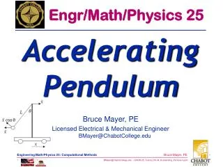
Accelerating Pendulum Demo – Problem 9.34 • For an Arbitrary Lateral-Acceleration Function, a(t), the ANGULAR Position, θ, is described by the (nastily) NONlinear 2nd Order, Homogeneous ODE q m W = mg • See next Slide for Eqn Derivation • Solve for θ(t)
N-T CoORD Sys Prob 9.34: ΣF = Σma • Use Normal-Tangential CoOrds; θ+ → CCW • Use ΣFT = ΣmaT
Prob 9.34: Simplify ODE • Cancel m: • Collect All θ terms on L.H.S. • Next make Two Little Ones out of the Big One • That is, convert the ODE to State Variable Form
Convert to State Variable Form • Let: • Thus: • Then the 2nd derivative • Have Created Two 1st Order Eqns
SimuLink Solution • The ODE using y in place of θ • Isolate Highest Order Derivative • Double Integrate to find y(t)
Θ with Torsional Damping • The Angular Position, θ, of a linearly accelerating pendulum with a Journal Bearing mount that produces torsional friction-damping can be described by this second-order, non-linear Ordinary Differential Equation (ODE) and Initial Conditions (IC’s) for θ(t): q m W = mg