Classic mapping technique
820 likes | 1.09k Views
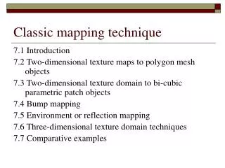
Classic mapping technique. 7.1 Introduction 7.2 Two-dimensional texture maps to polygon mesh objects 7.3 Two-dimensional texture domain to bi-cubic parametric patch objects 7.4 Bump mapping 7.5 Environment or reflection mapping 7.6 Three-dimensional texture domain techniques

Classic mapping technique
E N D
Presentation Transcript
Classic mapping technique 7.1 Introduction 7.2 Two-dimensional texture maps to polygon mesh objects 7.3 Two-dimensional texture domain to bi-cubic parametric patch objects 7.4 Bump mapping 7.5 Environment or reflection mapping 7.6 Three-dimensional texture domain techniques 7.7 Comparative examples
7.1 Introduction • The mapping technique • Techniques which store information in a 2D domain which is used during rendering to simulate textures. • Texture mapping • The mainstream application • Reflection mapping • Simulate ray tracing
7.1 Introduction • Environment mapping • Add pseudo-realism to shiny animated objects by causing their surrounding environment to be reflected in them. • Color mapping • Texture - does not mean controlling the micro-facets of the objects • controlling the value of the diffuse coefficients • Shading changes as a function of the texture maps.
7.1 Introduction • Three origins to the difficulties • How can we physically derive a texture value at a surface point if the surface does not exits. • How to map a 2D texture onto a surface that is approximated by a polygon mesh. • Aliasing problem
Possible ways to modulate a computer graphics model with a texture map • Color • Modulate the diffuse reflection coefficients in the local reflection model. • Specular color (environment mapping) • Special case of ray tracing • Normal vector perturbation (bump mapping) • Applies perturbation to the surface normal according to the corresponding value in the map. • Displacement mapping • Uses a height field to perturb a surface point along the direction of its surface normal. • Transparency • Used to control the opacity of a transparent object
Ways to perform texture mapping • Choice depend on • Time constraints • Quality of the image required • We will restrict the discussion to 2D texture maps. (Heckberts 1986) • 2D Texture mapping • 2D-to-2D transform • 2D texture object surface screen space • can be viewed as an image warping operation
Ways to perform texture mapping • Forward mapping • Two stages process • 2D texture space -> 3D object space • Parametrisation • Associates all points in texture space with points on the object surface • 3D object space 2D screen space • Projective transform • Inverse mapping • For each pixel we find its corresponding pre-image in texture space.
Two ways of viewing the process of 2D texture mapping (a) Forward mapping (b) Inverse mapping
7.2 Two-dimensional texture maps to polygon mesh objects 7.2.1 Inverse mapping by bi-linear interpolation 7.2.2 Inverse mapping by using an intermediate surface 7.2.3 Practical texture mapping
7.2.1 Inverse mapping by bi-linear interpolation • Inverse mapping • Consider a single transformation for 2D screen space (x,y) to 2D texture space (u,v). • An image warping, can be modelled as a rational linear projective transform: • We can write this in homogeneous coordinates as :
The inverse transform • If we have the association for the four vertices of a quadrilateral we can find the nine coefficients (a,b,c,d,e,f,g,h,i)
Bi-linear interpolation in screen space • Assuming vertex coordinate/texture coordinate for all polygons we consider each vertex to have homogeneous texture coordinates: • Use normal bi-linear interpolation scheme within the polygon, using homogeneous coordinates as vertices to give (u’,v’,q) for each pixel; then the required texture coordinates are give by:
7.2.2 Inverse mapping by using an intermediate surface • Used when there is no texture coordinate-vertex coordinate correspondence. • It can be used as a preprocess to determine the correspondence. • Two-part texture mapping: • To overcome the surface parametrisation problem • Introduced by Bier and Sloan (1986) • The intermediate surface must has an analytic mapping function.
Two-stage forward mapping process • First stage : S mapping • 2D texture space to 3D intermediate surface • Second stage : O mapping • 3D texture pattern onto object surface.
S mapping • Bier describes 4 intermediate surfaces • A plane at any orientation • The curved surface of a cylinder • The faces of a cube • The surface of a sphere • For example • Given a parametric definition of the curve surface of a cylinder as a set of points (,h) • c , d are scaling factors • θ0 and h0 position the texture on the cylinder of radius r.
Inverse mapping using the shrink wrap method Inverse mapping
Examples • Examples of mapping the same texture onto an object using different intermediate surfaces
7.2.3 Practical texture mapping • An example of a tank object texture being created from a photograph of a tank
Interactive texture mapping-painting in T (u,v) space 7.2.3 Practical texture mapping
7.2.3 Practical texture mapping • Agglomerating part maps into a single texture map.
7.3 Two-dimensional texture domain to bi-cubic parametric patch objects • The parametrization is trivial • P (u,v) T (s,t) • Catmull (1974) • Subdivide patch in object space, and at the same time subdivide corresponding texture in texture space. • Patch subdivision proceeds until it covers a single pixel • Cook (1987) • Object surfaces are subdivided into micro-polygons and flat shaded with values from a corresponding subdivision in texture space
7.3 Two-dimensional texture domain to bi-cubic parametric patch objects • Example
7.4 Bump mapping 7.4.1 A multi-pass technique for bump mapping 7.4.2 A pre-calculation technique for bump mapping
7.4 Bump mapping • Developed by Blinn in 1978 • An elegant device that enables a surface to appear as if it were wrinkled or dimpledwithout the need to model these depressions geometrically. • The only problem • Silhouette edge that appears to pass through a depression will not produce the expected cross-section
A one-dimensional example of the stages involved in bump mapping
The surface and its normal • Assuming the surface is defined by a bivariate parametric function P(u,v) • The surface normal on each point of the surface is then defined as • Pu and Pv are the partial derivatives lying in the tangent plane to the surface at point P
The displaced surface and it’s surface normal • The new displaced surface P’(u,v) • Two-dimensional height field B(u,v) called bump map • The new surface normal on P’
The partial derivatives of P’ and the new surface normal on P’ • The partial derivatives of P’ • If B is small we can ignore the final term so N’ become: • D is a vector lying in the tangent plane that pull N into the desired orientation and is calculated from partial derivatives of the bump map and the two vectors in the tangent plane.
7.4.1 A multi-pass technique for bump mapping • McReynolds and Blythe (1997) define a multi-pass technique. • They split the calculation into two components. The final intensity value is proportional to N’.L • First component : the normal Gouraud component • Second component : found from the differential coefficient of two image projections
A multi-pass technique for bump mapping (cont.) • To do this it is necessary to transform the light vector into tangent space at each vertex of the polygon. This space is defined by N, B, T • N is the vertex normal • T is the direction of increasing u (or v) in the object space coordiante system • B = N T • Normalised components of these vectors defines the matrix that transforms point into tangent space
A multi-pass technique for bump mapping (cont.) • Algorithm is as follows
7.4.2 A pre-calculation technique for bump mapping • Tangent space can also be used to facilitate a pre-calculation technique as proposed by Peercy et al. (1997) • It can be shown that the perturbed normal vector on tangent space given by
Example for bump mapping • A bump mapped object with the bump map
Example for bump mapping • A bump mapped object from a procedurally generated height field.
Example for bump mapping • Combining bump and color mapping • The bump and color map
7.5 Environment or reflection mapping • 7.5.1 Cubic mapping • 7.5.2 Sphere mapping • 7.5.3 Environment mapping : comparative points
7.5 Environment or reflection mapping • Originally called reflection mapping • Suggested by Blinn (1977) • Consolidated into mainline rendering techniques in an important paper in 1986 by Greene • Used to approximate the quality of a ray-tracer for specular reflections • It is a classic partial offline or pre-calculation technique • V Rv M(Rv)
7.5 Environment or reflection mapping • Example
Disadvantages • Correct only when the object becomes small with respect to the environment that contains it. • An object can only reflects the environment– not itself. • A separate map is require for each object. • A new map is required whenever the view point changes
Three methods for environment mapping • Cubic mapping • Latitude-longitude mapping • sphere mapping
7.5.1 Cubic mapping • A problem of a cubic map is that if we are considering a reflection beam formed by pixel corners, or equivalently by reflected view vectors at a polygon vertex , the beam can index into more than one map.