S.I. Dimitriadis , N.A. Laskaris , A. Tzelepi

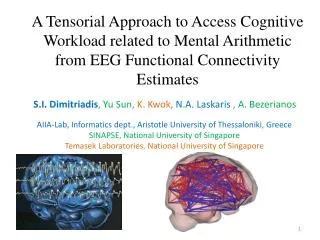
1. Go with the winner: optimizing detection of modular organization differences in dynamic functional brain networks S.I. Dimitriadis, N.A. Laskaris, A. Tzelepi AIIA-Lab, Informatics dept., Aristotle University of Thessaloniki Electronics Laboratory, Department of Physics,University of Patras ICCS, National Technical University of Athens

2. Outline • Introduction • -Various studies examined modular organization based on • numerous measures of neural synchrony • -It is not known yet how to quantify the employed descriptors in • terms of functional community structure Methodology We introduced a framework for detecting the synchronization measure that best describes and differentiates two conditions (or two groups of subjects) in terms of time-varying functional communities Results Conclusions

3. A great variety of measures has been proposed to quantify neural synchrony An important question is whether the detection of modules is influenced by the adopted synchronization measure and also by the clustering algorithm (Pavan & Pelillo,2007). An additional question is whether the distribution and also the number of modules in healthy and impaired subjects are similar or not

4. Motivation and problem statement The vast majority of previous studies have been based on analyzing the topological properties of static graphs -Inaccuracies can be more severe for fast-recordingmodalities, in particular for EEG/MEG and to a lesser extent for fMRI. To alleviate the above limitations, we used time–varying graphs, which describe temporally evolving networks that have fixed nodes but changeable links Our motivation was to present a method to qualify the employed descriptors in terms of the resulting functional community structure

5. Outline of our methodology We introduced a framework for detecting the synchronization measure that best describes and differentiates two conditions Time-varying functional communities Specifically, we considered the multichannel EEG recordings during an attentive and passive eye movement task as observations from two different states of the (same) brain, Discriminability was measured for different types of coupling (linear vs. nonlinear) and different forms of covariation (amplitude/phase)

6. Data acquisition: Visual ERP experiment 5 subjects 64 EEG electrodes Horizontal and Vertical EOG Trial duration: 5.5 seconds 2 runs, 50 trials for each condition • 2 Conditions: • Attentive • Passive • (Left/right)

7. Exploratory Analysis – Contrast function Two different sets of patterns/objects {Xi} and {Yj} can be compared in three steps. We first established an appropriate pairwise dissimilarity measure D(Xi,Yj). This measure is then applied to all possible pairs to compute the inter-set scatter (IS ATTENTIVE - PASSIVE) and the two within-set scatters (WS ATTENTIVE and WS PASSIVE). The computed quantities are finally combined to express the set difference,as follows:

8. Statistical approach of J-index The statistical significance of a specific value for the J-index can be calculated based on a randomization procedure. We first splitting the objects (i.e., all EEG-traces from attentive and passive conditions) at random into two groups and repeating the computations for J multiple times to form a baseline distribution for the J-index indicative of random partitioning (e.g.10.000 -> P < 0.001) Finally, the original value of the J-index is compared to the derived baseline distribution, and this comparison is expressed via a P-value

9. Quantify communities differences Adopting a synchronization measure, we estimated the connectivity strength for each pair of signals The set of patterns of the attentive task, at each latency t, can be compared against the set of patterns of the passive task Graph partition algorithm N N 1 2 3 2 1 ….. 2 1 3 2 1 2 3 1 2 …. 2 1 3 2 2 3 4 1 2 … 1 2 3 2 2 2 3 1 2 … 1 2 2 2 Attentive Task Passive Task

10. Adjust J-index to community differences We adopted VI (Variation of Information) as a dissimilarity measure to quantify community differences Suppose we have two clusterings X and Y. X=[1 1 2 1 , … 2 1] & Y=[1 3 2 1 , … 2 3] Then the variation of information between two clusterings is: Where H(X) is the entropy of X and MI(X,Y) is the mutual information between X and Y (Meila, 2007)

11. Adjust J-index to community differences N Numerator & Denominator = J-index

12. Adjust J-index to dynamic community differences Using the latency-dependent measurements Jt and the associated p-values (produced via trial-shuffling) derived for each subject separately, we summarize the comparison between attentive and passive task by means of the TICDI (Time-Integrated Community Difference Index ) where Ns denotes the number of subjects and NT the total number of discrete time points (latencies)

13. Τhe functional connectivity graph (FCG) describes coordinated brain activity To accommodate the various aspects of neural synchrony, we employed different functional connectivity estimators. Coherence (COH), Mutual Information (MI), Phase Locking Value (PLV), Phase Lag Index (PLI) and weighted – Phase Lag Index (wPLI) Every estimator takes as input a pair of time series recorded at distinct sites and derives an estimate of the strength for the corresponding functional interaction Such an interaction can have either linear or nonlinear characteristics and can take the form of either amplitude or phase covariation

14. Time – varying FCGs We employed a frequency-dependent criterion to define the width of the time-window (Dimitriadis et al., 2010) . Using a regular time step, the centre of the window was moved forward, and the whole network connectivity was re-estimated based on the new signal segments Each FCG was defined by the (time dependent) [64 × 64] matrix W(t) with entries the pairwise coupling strengths FCG (u(t),v(t)) derived based after integration within the 4–10 Hz frequency range. FCG -> TVFCGs

15. Detecting Significant Couplings Significant values were determined after calculating connectivity strength for surrogates derived by randomizing the order of trials in one of the channels of each pair Significance levels were then extracted from the p-values of the difference between synchronization estimates in the original and surrogate data (e.g.1.000 -> P < 0.01) Significance probabilities were corrected using the FDR method in order to correct for multiple comparisons The expected fraction of false positives was restricted to q ≤ 0.01

16. Task-induced differences in functional segregation (TICDI) The ranking of synchronization measures according to TICDI was: COH < MI < PLI < WPLI < PLV

17. Functionally Segregated Patterns Evolution of clusterings across trials and subjects between attentive (A) and passive condition (P) in a) left and b) right presentation The most important trend is that during the attentive condition, the number of functional groups that are emerging is higher compared to the passive condition.

18. Participation Index identified functional hubs Participation Index is a feature of each nodes connectivity relative to the modularity decomposition of the entire network. We define the participation coefficient PI of node i as: where is the sum of weights (links) of node i to nodes in module s, is the total strength of node i and is the total number of modules. The participation coefficient of a node is therefore close to one if its links are uniformly distributed among all the modules and zero if all its links are within its own module

19. Participation Index identified functional hubs In order to detect hubs across time and subjects,weranked PI values for each network and then we keep the indices of the nodes belonging to the 20% of the highest values Sensors belonging in at least 80% of latencies at each subject and to the 20% highest PI-values of each network were defined as hubs on a group level • Our analysis was divided into three parts: • the baseline period, ([-1 0] sec), • the period from the onset of the stimulus until the weakening of the Visual Evoked Potential (VEP) ([0 0.2] sec) and • the eye – movement preparatory period until the initiation of the antisaccade (attentive condition) ([0.2 3.5]sec).

20. Brain rhythm interpretation In the present study, we analyzed EEG signals in the frequency range of 4 – 10 Hz including both θ and lower-α (α1). Both brain rhythms were found to be involved in attentional processes (von Stein and Sarnthein, 2000 ; Sauseng et al., 2005)

21. Participation Index identified functional hubs The extension of hubs : (a)bilaterally over frontal regions and also (b)over parieto-occipital sites contralaterally to the presentation of the stimulus, an observation that can be attributed to attention and also to preparatory effects of the motor system preceding antisaccades ( Buschman and Miller, 2007 ; McDowellet al., 2005)

22. Conclusions Our methodology offers a novel framework for optimizing the detection of Functional brain organization between two conditions (or groups) using the notion of dynamic functional brain networks In the future, we will apply the methodology to data from other other neuroimaging techniques as well (e.g., MEG, fMRI, MRI, DTI) and also to source reconstruction techniques The incorporation of causality measures and the replacement of the over-simplifying notion of pairwise interactions with multivariate synchrony should be considered in the future.

23. Further directions Fusion of Fc estimators with different weight for Constructing an aggregated FCG ?

24. References [1] S.I.Dimitriadis, N.A. Laskaris, V.Tsirka, M.Vourkas, S.Micheloyannis and S.Fotopoulos,” Tracking brain dynamics via time-dependent network analysis,” Journal of Neuroscience Methods, vol.193,pp.145-155,2010. [2] Meila M (2007) Comparing clusterings-an information based distance. J Multivariate Anal 98:873–895 [3]A. Von Stein and J. Sarnthein J, “Different frequencies for different scales of cortical integration: from local gamma to long-range alpha/theta synchronization,” Int. J. Psychophysiol., vol.38, pp.301–313,2000. [4]P. Sauseng,W.Klimesch, W.Stadler, M. Schabus,M. Doppelmayr M, S. Hanslmayr,W.R. Gruber and N. Birbaumer N, “A shift of visual spatial attention is selectively associated with human EEG alpha activity,” Eur. J. Neurosci. vol.22, pp.2917–2926, 2005. [5] T.J.Buschman, and E.K. Miller, “Top-down versus bottom-up control of attention in the prefrontal and posterior parietal cortices,” Science., vol.315, pp.1860–1862,2007. [6] J.E. McDowell,J.M. Kissler, P.Berg, K.A.Dyckman,Y. Gao, B. RockstrohB,et.al.,”Electroencephalography/magnetoencephalography study of cortical activities preceding prosaccades and antisaccades,”NeuroReport, vol.16, pp.663–668,2005. [7]Pavan M, Pelillo M (2007) Dominant sets and pairwise clustering. IEEE Trans PAMI 29(1):167–172