
Regression in GRID
E N D
Presentation Transcript
Regression in GRID FE423 - February 27, 2000
Labs • Another reason for AML - re-sampling • resample big grid to little grid • do lab on little grid • work out bugs on little grid • write up aml • check aml on little grid • run aml on big grid while writing up lab • Send me a note when you finish your lab
Outline • Probability models - simulation • Linear models - regression • Logistic Regression • Answering questions with data
Questions In forest management, we have questions like: • Does logging cause landsliding? • Does logging impact fish?
Spatial Data One tool for answering them is spatial data. • Outcomes • fish counts, landslides, sediment supply, etc. • Management Activities • harvest units, roads, etc. • Other things that might impact • slope, contributing area, etc.
Natural Variability Unfortunately, natural processes are highly variable, so we rarely have a 1-to-1 causal relationship. Management impacts are usually small compared to the natural variation. In competitive ecosystems, a small impact can be the difference in survival.
Probability Models in GRID We can model this natural variability in GRID with random functions • RAND() • NORMAL()
The RAND() Function The RAND() function makes draws from the range (0,1)
Simulating Random Events Example: We can use SMORPH hazard ranking to simulate landslide observations. haz = con(slope < 40 and plan < .5, 1, ~ ... prob = con(haz eq 0, .001, haz eq 1, .01, .1) LS_sim = con(rand() < prob, 1, 0)
Simulating Random Events Planform curvature slope Simulated landslides hazard
The NORMAL() Function The normal() function makes draws from standard normal distribution
Simulating Random Events Example: fish counts we can model observations fish = 40 + 10 * normal() and include physical inputs fish = 20+stand_age+10*normal()
Regression Overview Just like prediction, but in reverse. Start with fish = 20+age+10*normal() but, let’s say we don’t know the parameters fish = a+b*age+e*normal() We should use coverages FISH and AGE to get the model parameters a, b, and e. ‘b’ tells us how many more fish we will get if we keep older stands along the stream.
Plotting Relationships Plotting in GRID is done through Stacks. MAKESTACK <stack> LIST <grid ... grid> STACKSCATTERGRAM <stack>
Regression in GRID In doing regression in GRID we: • make a SAMPLE file • Grid: samp1 = sample(maskgrid, ing1, ing2) • do REGRESSION on it • Grid: regression samp1
The SAMPLE Function SAMPLE(<mask_grid>, {grid, ..., grid}) SAMPLE(<* | point_file>, {grid, ..., grid}, {NEAREST | BILINEAR | CUBIC}) Arguments <mask_grid> - the grid which defines the cells to sample. Cells in the mask grid with valid values will be sampled. {grid, ..., grid} - the name of one or more grids whose values will be sampled based upon the mask grid. <*> - allows for the interactive graphical input of the input sample points. The grid specified by {grid} should to be displayed for reference. <point_file> - the name of the ASCII text file containing coordinates of points to be sampled. <NEAREST | BILINEAR | CUBIC> - specifies the resampling algorithm to be used when sampling a grid. It is used only when point coordinates are entered as input. See Resampling grids for a description of the resampling methods. NEAREST - nearest neighbor assignment. BILINEAR - bilinear interpolation. CUBIC - cubic convolution.
The REGRESSION Command REGRESSION <sample> {LINEAR | LOGISTIC} {DETAIL | BRIEF} Arguments <sample> - the name of the input file which can be created using the SAMPLE function. {LINEAR | LOGISTIC} - keywords specifying the type of regression to be performed. LINEAR - linear regression with least square fit estimation is performed. LOGISTIC - logistic regression with maximum likelihood estimation is performed. {DETAIL | BRIEF} - keywords specifying whether a full or abbreviated report will be displayed on a screen. DETAIL - displays a fully detailed report, the result of running the regression model. BRIEF - displays the values of coefficients, RMS Error and Chi-Square only.
Regression in GRID Grid: samp1 = sample ( maskgrid, ing1, ing2 ) Grid: &sys cat samp1 1 1.5 3.5 1 0.1 0 2.5 3.5 1 0.2 0 3.5 3.5 0 0.5 2 0.5 2.5 3 0.75 0 1.5 2.5 3 0.9 3 2.5 2.5 1 1 3 3.5 2.5 2 2 0 0.5 1.5 MISSING -0.1 0 1.5 1.5 0 -0.25 3 2.5 1.5 0 -1 2 3.5 1.5 2 0 1 0.5 0.5 3 0.707 1 1.5 0.5 2 0.866 0 3.5 0.5 0 MISSING Grid: regression samp1 coef # coef 0 1.250 1 -0.029 2 0.263 point id z z error 1 1.000 -0.248 2 0.000 -1.274 3 0.000 -1.381 4 2.000 0.639 5 0.000 -1.400 6 3.000 1.516 8 0.000 -1.184 9 3.000 2.013 10 2.000 0.808 11 1.000 -0.350 12 1.000 -0.420 RMS Error = 1.166 Chi-Square = 16.307
Regression in GRID fish = 20 + stream_age + 10 * normal() Grid: samp = sample(fish,stream_age) List grids ... 100% Grid: regression samp linear brief coef # coef ------ ---------------- 0 19.436 1 1.000 ------ ---------------- RMS Error = 9.983 Chi-Square = 3064046.998
Regression on Non-linear Models Linear regression on non-linear models doesn’t always give the ‘correct’ results, even on coefficient signs. Grid: fish = ln(age) + ln(fa) - ln(gradient) Grid: sumple = sample(fish, age, fa, gradient) Grid: regression sumple linear brief coef # coef 0 6.023 1 0.019 2 0.000 3 -0.105 RMS Error = 1.453 Chi-Square = 3335.795 Correct sign Incorrect sign Correct sign
Logistic Regression Regression on zeros and ones makes it hard to fit a line. We can however do regression on the probability. ls = con(rand() < prob,1,0) prob = 1/(1+exp(-a0-a1*x1-a2*x2…))
Logistic Regression: Example Grid: ls = con(curve < 0 and slope > 40,1,0) Grid: s_ls = sample(ls, slope , curve ,aspect) Grid: regression s_ls logistic brief coef # coef 0 -25.321 1 0.507 2 -16.508 3 0.000 RMS Error = 0.094 Chi-Square = 366.098
Answering Questions • Map your data and look • Plot your data • make a stack • make a stack scattergram • adjust scale to fit one-to-one • Regression • sample • regression
Answering Questions 1. Are these landslides aspect dependent? Can you prove that?