Download
1 / 19
190 likes | 303 Views
Fleet dynamics of the SW Indian Ocean tuna Fishery : a bioeconomic approach Main results September 2013 C. Chaboud. Main characteristics of model. Resources. Three main tuna species : skipjack (SKJ), yellowfin tuna (YFT), big eye tuna (BET) and albacore (ALB)

E N D
Fleet dynamics of the SW Indian Ocean tuna Fishery : a bioeconomic approach Main results September 2013 C. Chaboud
Resources • Three main tuna species : skipjack (SKJ), yellowfin tuna (YFT), big eye tuna (BET) and albacore (ALB) • Migrating and straddling socks between EEZ’s and international waters • Seasonal spatial repartition varying among species and age (differences between adults and juveniles) • Most species are long living species
Fleets • Fishing methods: purse seines (FADs + free schools), bait boats, longlines and gill nets. • Differences in costs , in impacts on resource components by species or by age (catchability) , in targeted markets and hence in prices • Different countries or group of countries owning or exploiting tuna resources • Fleets = sets of boats, defined by fishing methods and countries, and specific prices. • Spatial fleet behavior (developed later)
Modeling choices • Time step : month • Simulation length : up to 25 years • Age structured model (by month) • Threespecies (SKJ, BET, YFT) • Muti gears • Three types of countries or owning and/or exploiting the resource • Pure owners countries (don’t’ significantly exploited the resource • Pure foreign fishing countries (no resource in the region) • Owners and fishing countries
Modeling choices • Spatially explicit model : resources and fleets are redistributed a each time step • Different “layers” showing • legal or technical constraints for access to resources • Resources • Fleets dynamics • Position of harbors (fleets bases) • exploitation results • Distribution of exploitation results between fishing and resource owners countries. • Model can be used in a reduced form (limited number of species, gears, fishing countries, cells…)
The grid • 12 lines x 19 Columns • 228 square cells 5° X 5 °
EEZs and legalboundaries layerManycells are shared by differentEEZs
Modeling choices • Market : two possibilities • Fishery is price taker(realistic for an isolated or limited exploitation system. Exogenous prices are defined by species, age (juveniles-adult) and fishing gear) • Inverse demand function P = P(Q) (realistic if there is some coordination between all Tuna RFMOs for catch restriction or capacity control). • Cost functions specified by fleet • Fixed cost : insurance, depreciation, maintenance, fishing license fees… • Variable costs : • energy, food (linked to time at sea) • labor (linked to yield value) • royalties paied for access (linked to quantities …)
Resource • Structured by age (age class = model time step = month) • Catchability defined par species, gear and live stage (juvenile, adult) • Von Bertalanffy growth curves, • Natural mortality specified by age • Different possibilities for recruitment • Independent of dependent (hockey stick shaped) of fecund biomass • Deterministic or stochastic (month and year effects)= • Spatial monthly repartition per species and life stage (juvenile/adult) is due to • 1. by a spatial preference matrix SP (different for adults and juveniles) and a spillover from each cell to adjacent cells. Sp can be modified during simulations to introduced changes in spatial preference • 2. spillover : at each time step a constant part of each cell is redistributed to adjacent cells.
Spatial and temporal resource behavior • At every time step resource Na (stock per species in number per age a ) less catch Ca and natural mortality Ma , is redistributed according to a spatial preference matrix SPaij, defined per month, species and life stage , . Total stock Cellij time t Cellij time t +1
Spatial and temporal resource behavior • After the computation on the resource dynamics in number • The biomass is obtained (for a species, a cell i,j and at age a) : • The value of biomass is now computed, given an price vector by age (for a species) : • Biomass values is used as input in the economic module of the model.
Spatial temporal Fleets behavior • The total number of boats per fishing fleet (defined par a type of gear for a given country) can follow two types of time behavior • Exogenous defined (fixed or varying during the simulation) • Endogenous entry/exit behavior at the beginning of each year (ie every 12 time steps), depending from past year fleet cumulated profit (Smith model, 1968) :
Spatial temporal Fleets behavior : a free ideal distribution approach • Two steps method : 1 )Fleets are first distributed among harbors, and 2 ) from harbors to cells • Past characteristics (“value”) of cells are computed • Biomass value of the cell in t-1 and t-12 • Revenue per boat per cell in t-1 and t-12 • Catch per boat per cell in t-1 and t-12. • Profit per boat per cell in t-1 and t-12
Spatial temporal Fleets behavior : a free ideal distribution approach We compute first the « absolute value Of harbors (1) and then their « relative value » (2) which is their attractiveness h : harbor, b : fishing method, p : fishing country v = cell value dist= distance between harbor and cell Then each fleet is distributed between harbors (3)
Spatial temporal Fleets behavior : a free ideal distribution approach Then we compute the absolute (1) and relative (2) attractiveness for each cell cellule, for each fishing country (p), fishing method (b) and harbor (h) The boats can now be distributed between cells (3)
Spatial temporal Fleets behavior • Particularity of the purse seine fishery : at each time step, the purse seine fleets are divided into two strategic components ‘Purse seines FAD’ and ‘Purse seines Free Schools’ according their relative economic results in t-1. The variation of the total number of purse seines of one fleet at the beginning of year y is obtained by adding their respective economic cumulated results (profit) over the past year.
Model outputs • Biomass per species, cell, age, EEZ (in volume and value). • Catches per species, age, fleet, fishing country, EEZ . • Private profit per fleet. • Current and discounted rent (NPV) per fishing and owners countries. • Fleet number and spatial distribution • Economic rent for states (private profit + net state incomes) current and discounted (NPV).
Control variables (defined before simulation) • Initial fleet numbers (with possibility of effort multiplier varying during simulation) • Fees and royalties • MPA location (one or several adjacent or not grid cells) • Control of access by resource owners (ie fishing agreements) • Quotas , total or per ZEE (to be developped)