Download

1 / 106
1.08k likes | 1.32k Views
Resource Markets. Remember that the following terms are just different words for the same things. Resources Inputs Factors of Production Whichever they’re called, they are things that are used to produce output.

E N D
Remember that the following terms are just different words for the same things. • Resources • Inputs • Factors of Production • Whichever they’re called, they are things that are used to produce output.
Input and output markets can be perfectly competitive or not. So there are four possibilities.
A firm uses inputs to produce outputs. So there are four possibilities.
A firm uses inputs to produce outputs. So there are four possibilities.
A firm uses inputs to produce outputs. So there are four possibilities.
A firm uses inputs to produce outputs. So there are four possibilities.
Input Market Possibilities • Perfect Competition – many buyers of the input with no influence on the input price • Monopsony – one buyer of the input • Oligopsony – a few buyers of the input • Monopsonistic Competition – many buyers but with some influence over input price • Perfect Competitors have a horizontal input supply curve. • Monopsonists, oligopsonists, & monopsonistic competitors face an upward sloping input supply curve.
P P S D P* P* D Q Q Q* W W S S W* W* D L L L* Industry Perfectly Competitive Firm Output or Product Input or Labor
Derived Demand • Because the demand for an input is derived from the demand for the output that it is used to produce, the demand for an input is called a derived demand.
To determine how much input a firm will use, we need a few concepts.
If a firm hires all workers at the same wage, then the total resource cost (TRC) or total cost of labor (TCL) is • the wage per unit of labor times the amount of labor hired. • TRC = TCL = W•L
Marginal Resource Cost (MRC) • the change in total variable cost that results from the employment of an additional unit of an input. • MRC = TVC / L = dTVC/dL
Average Resource Cost (ARC) • the total variable cost per unit of input • ARC = TCL / L • If the firm hires all workers at the same wage, then • ACL or ARC = TCL / L = (W•L)/L = W
Marginal Physical Product (MPP) or Marginal Product (MP) • the change in the quantity of output that results from the employment of an additional unit of an input. • MPP = DQ /DL = dQ/dL
Marginal Revenue Product (MRP) • the change in total revenue that results from the employment of an additional unit of an input. • MRP = DTR /DL = dTR/dL
What is the difference between MPP & MRP? • Suppose your company produces chairs. • The MPP tells how many more chairs you can make if you hire another worker. • The MRP tells how much more revenue you can make from the additional chairs produced by the additional worker.
Alternative formula for MRP • MRP = DTR = DTRDQ DL DL DQ • = DTRDQ DQ DL • = MR . MPP • So, MRP = MR . MPP
Sales Value of the Marginal Product (SVMP) or Value of the Marginal Product (VMP) • the price of the output multiplied by the marginal physical product of the input. • VMP = P . MPP
Recall: If a firm is a perfect competitor in the product market, marginal revenue is equal to the price of the output (MR = P). • Then, MRP = MR . MPP • = P . MPP • = VMP • So, MRP = VMP • for a firm that is a perfect competitor in theproduct market.
Recall: If a firm is a not perfect competitor in the product market, marginal revenue is less than the price of the output (MR < P). • Since MRP = MR . MPP • and VMP = P . MPP, • MRP < VMP, • for a firm that is not a perfect competitor in the product market.
If a firm is perfectly competitive in the product market, then MRP = VMP. If a firm is not perfectly competitive in the product market, then MRP < VMP.
Example: A firm sells its shirts in a perfectly competitive product market for $10 each.LQ 0 0 10 70 20 130 30 180 40 220 50 250 60 270 70 280
Example: A firm sells its shirts in a perfectly competitive product market for $10 each.LQMPP=DQ/DL • 0 0 • 10 70 • 20 130 • 30 180 • 40 220 • 50 250 • 60 270 • 70 280 --- 7 6 5 4 3 2 1
Example: A firm sells its shirts in a perfectly competitive product market for $10 each.LQMPP=DQ/DLTR=PQ • 0 0 --- • 10 70 7 • 20 130 6 • 30 180 5 • 40 220 4 • 50 250 3 • 60 270 2 • 70 280 1 0 700 1300 1800 2200 2500 2700 2800
Example: A firm sells its shirts in a perfectly competitive product market for $10 each.LQMPP=DQ/DLTR=PQMR =DTR/DQ • 0 0 --- 0 • 10 70 7 700 • 20 130 6 1300 • 30 180 5 1800 • 40 220 4 2200 • 50 250 3 2500 • 60 270 2 2700 • 70 280 1 2800 --- 10 10 10 10 10 10 10
Example: A firm sells its shirts in a perfectly competitive product market for $10 each. MRP =DTR/DLLQMPP=DQ/DLTR=PQMR =DTR/DQMRP= MR•MPP 0 0 --- 0 --- 10 70 7 700 10 20 130 6 1300 10 30 180 5 1800 10 40 220 4 2200 10 50 250 3 2500 10 60 270 2 2700 10 70 280 1 2800 10 --- 70 60 50 40 30 20 10
Focusing on the first and last columns of the previous table, we have the MRP schedule.LMRP • 0 --- • 10 70 • 20 60 • 30 50 • 40 40 • 50 30 • 60 20 • 70 10
Plotting points we have a graph of the MRP curve. MRP 70 60 50 40 30 20 10 MRP labor 0 10 20 30 40 50 60 70
Suppose we want to maximize our profits. How much input we should use? • MRP > MRC employ more input • MRP < MRC cut back employment • MRP = MRC profit-maximizing employment level
W SL = MRC = ARC L The Perfectly Competitive Labor Market Firm Each time a firm hires another unit of labor, its cost increases by the price of the labor (W). So for a firm in a perfectly competitive labor market, MRC = W . (If a firm is not in a perfectly competitive labor market, this isn’t true.) Also, remember that the supply curve of labor for a firm that is perfectly competitive in the labor market is a horizontal line at the going wage W. Recall that for a firm that hires all workers at the same wage, ARC = W. So for a firm that is perfectly competitive in the labor market, MRC, ARC, and SLare all the same horizontal line at the wage W.
Suppose the firm in the example we considered earlier is also perfectly competitive in the labor market. • So the MRC is the same as the price of labor or the market wage. • Let’s see what the demand curve for labor is for this firm. • Let’s first assume that other inputs are fixed. • What we need to know is how many workers will be hired at various wage levels.
Remember: You hire workers as long as they add at least as much to revenues as they add to cost. • Suppose the market wage is $70. How many workers will you hire? • 10 • Suppose the market wage is $60. How many workers will you hire? • 20 • Suppose the market wage is $50. How many workers will you hire? • 30 • Suppose the market wage is $40. How many workers will you hire? • 40 LMRP 0 --- 10 70 20 60 30 50 40 40 50 30 60 20 70 10
Remember we have been trying to determine what the demand curve for labor looks like for this firm. • All of our demand curve points have been points on the MRP curve. • The demand curve for labor by the firm is just (the downward sloping part of) the MRP curve.
A Firm’s Demand Curve for Labor $ 70 60 50 40 30 20 10 demand curve for labor labor 0 10 20 30 40 50 60 70
In the last few slides, we were assuming that inputs other than labor were fixed. • Suppose now that all inputs are variable; we are in a long run situation. • When the wage decreases, firms will adjust their usage of other inputs, such as capital. • When the wage dropped, the cost of production fell. So the firm would probably produce more and would therefore need more capital. • However, they may use less capital, substituting the now less expensive labor input. • So, when the price of an input drops, the amount used of other inputs may increase, decrease, or remain the same.
Suppose that when the wage falls from W1 to W2, the amount of capital used increases from K1 to K2. When labor has more capital with which to work, labor is more productive. So the MRPL is greater. Therefore, the demand curve is derived from parts of different MRPLs. When capital can not be changed, the quantity of labor demanded (in response to the wage drop) only increases from L1 to L’. When capital can be changed, the quantity of labor demanded increases to L2. $ W1 W2 DL MRPL2 (amt of capital is K2) MRPL1 (amt of capital is K1) L1 L’ L2 labor
Substitution & Output Effects of a change in wage Suppose that at the initial wage, the firm is operating at point A, the tangency of isocost 1 and isoquant 1. The slope of an isocost is –PL / PK = -W / PK , so when the wage falls, the isocosts become flatter. Capital The firm moves to point B, the tangency of isoquant1 with the flatter isocost2a, substituting away from capital and toward labor. Then since production has become less costly, the firm moves out to point C. It has moved out along the expansion path to the tangency between isoquant2 and isocost2b (which is parallel to isocost2a). expansion path Isocost 1 C A Isoquant 2 Isocost 2a B Isocost 2b Isoquant 1 Labor
Substitution & Output Effects of a change in wage The movement from A to B represents the substitution effect. The firm uses more labor and less capital, since labor has become relatively cheaper. The movement from B to C is the output effect. The firm uses more labor and more capital, at C than at B, since it has expanded production in response to the drop in the cost of production. The combined effect is to use more labor in response to the wage drop. In this particular graph, the combined effect on capital is to use slightly more capital. (C is higher than A.) Capital expansion path Isocost 1 C A Isoquant 2 Isocost 2a B Isocost 2b Isoquant 1 Labor
However, in response to a drop in the wage, the amount of capital used may increase if the output effect is larger than the substitution effect, decrease if the output effect is smaller than the substitution effect, or remain the same if the output effect is the same size as the substitution effect. Capital expansion path Isocost 1 C A Isoquant 2 Isocost 2a B Isocost 2b Isoquant 1 Labor
Let’s start with the DL and a wage of W1. (Suppose the price of the product is 100.) When the wage (or price of an input) falls, firms increase production. The increase in industry supply drives down the price of the product (perhaps to 80). This reduces VMPL = P·MPPL which is also DL = MRPL = MR·MPPL. So the DL decreases or shifts leftward. So instead of just adding up the individual firms’ DLs, the industry demand curve for labor consists of points from different ΣDLs. A perfectly competitive industry’s demand for labor wage The Industry wage The Firm DL W1 W1 ΣDL1 (P = 100) DL1 (P = 100) W2 W2 ΣDL2 (P = 80) DL2 (P = 80) L1 L2 L1 L2 labor labor
4 major determinants of an industry’s elasticity of demand for labor with respect to its wage • Price elasticity of demand for the product. • Ease of substitution of one input for anotherin the production process. • Elasticity of supply of other inputs. • The amount of time allowed for adjustment to the change in wage.
1. Price elasticity of demand for the product. Suppose the wage increases. That will drive up the price of the product. If the demand for the product is very responsive (or elastic) to price increases, the quantity demanded of the product will decrease considerably. The quantity demanded of labor will therefore also decrease considerably. So the more elastic the demand for the product is with respect to its price, the more elastic the demand for labor will be with respect to its wage.
2. Ease of substitution of one input for another in the production process. Again suppose the wage increases. If it is easy to substitute another input for the labor whose wage has increased, firms will reduce considerably the quantity of labor whose wage has gone up. So the easier substitution is, the greater the elasticity of demand for labor with respect to its wage will be.
3. Elasticity of supply of other inputs. Again suppose the wage increases. Suppose also that the supply of other inputs is very responsive (elastic) to the prices of those inputs. Then when firms start looking for alternative inputs to substitute for the labor that has become more expensive, it won’t take a very large increase in the price of the alternative inputs to bring about a large increase in the supply of those inputs. So it will not be very costly to switch to other inputs and the firms will be able to cut back on the labor quite a bit. So the greater the elasticity of supply of alternative inputs, the greater the elasticity of demand for labor.
4. The amount of time allowed for adjustment to the change in wage. One more time, suppose the wage increases. When firms have more time to adjust to the change, more options may become available. For example, new machines may be developed to do the work that the now more expensive labor is doing. So firms will be able to cut back more on their labor usage. So the more time allowed for adjustment, the greater the elasticity of demand for labor.
Market demand for labor (accountants, for example) • To determine the demand curve for accountants, we just horizontally sum the various industry demand curves for all the industries that hire accountants.
The shape of the supply curve of an input depends on the specific case. The supply curve to one industry will be flatter (more elastic) than the supply curve to the economy as a whole. The smaller the share of the total market accounted for by a particular industry, the more elastic its input supply curve. The supply curve to an individual firm in a perfectly competitive input market will be horizontal (perfectly elastic).