Download
1 / 68
680 likes | 738 Views
Parallelism & Algorithm Acceleration. M. Wijtvliet Embedded Computer Architecture 5KK73. But first …. Thursday: handout GPU assignment How many of you have laptop with OpenCL or CUDA capable video card?. Today’s topics. The importance of memory access patterns

E N D
Parallelism & Algorithm Acceleration M. Wijtvliet Embedded Computer Architecture 5KK73
But first … • Thursday: handout GPU assignment • How many of you have laptop with OpenCL or CUDA capable video card?
Today’s topics • The importance of memory access patterns • Vectorisation and access patterns • Strided accesses on GPUs • Data re-use on GPUs and FPGA’s • Classifying memory access patterns • Berkeley’s ‘7 dwarfs’ • Algorithmic species • Algorithmic skeletons • Algorithmic skeletons for accelerators 5KK73 |Slides: C. Nugteren
Vector-SIMD execution SIMD processes multiple scalar operations concurrently ld r1, addr1 ld r2, addr2 add r3, r1, r2 st r3, addr3 for (i=0; i<N; i++) c[i] = a[i] + b[i]; ldv vr1, addr1 ldv vr2, addr2 addv vr3, vr1, vr2 stv vr3, addr3 N iters N / 4 iters 5KK73 | Slides: C. Nugteren
Vector-SIMD execution A single instruction being executed: • By multiple processing engines (ALUs, PEs, cores, nodes) • Concurrently in lockstep (no synchronization) • On multiple data elements Present in a wide range of architectures • SIMD, GPU, AVX, SSE, NEON, Xetal, etc. Type of parallelism that is easy and cheap to implement • No coherence problem • No lock problem Caveat: Hard to program and/or easy to lose many factors of performance 5KK73 | Slides: C. Nugteren [Slides taken from P. Sadayappan]
How to use SIMD instructions? Pick your favourite: • Vectorising compiler (ICC, latest GCCs) • Macros or intrinsics • Assembly for (i=0; i<N; i++) c[i] = a[i] + b[i]; __m128 rA, rB, rC; for (inti = 0; i <N; i+=4) { rA = _mm_load_ps(&a[i]); rB = _mm_load_ps(&b[i]); rC = _mm_add_ps(rA,rB); _mm_store_ps(&C[i], rC); } ..B8.5 movaps a(,%rdx,4), %xmm0 addps b(,%rdx,4), %xmm0 movaps %xmm0, c(,%rdx,4) addq $4, %rdx cmpq $rdi, %rdx jl ..B8.5 5KK73 | Slides: C. Nugteren [Slides taken from P. Sadayappan]
What is the performance impact? Properties of the example: • Stride-1 accesses to array a • Inner loop has independent operations (no loop carried dependences) • Array a resides in L1 cache (12.5 KB) Performance in GOPS/s on 128-bits wide CPU: for (i=0; i<N; i++) a[i] = a[i] + 1; 5KK73 | Slides: C. Nugteren [Slides taken from P. Sadayappan]
Strided accesses (1/2) Properties of the example: • Stride-16 accesses to array a • Inner loop has independent operations • Array a resides in L1 cache Performance in GOPS/s on 128-bits wide CPU: for (i=0; i<N; i+=16) a[i] = a[i] + 1; Why no performance gain? • Operands are not contiguous in memory • Multiple loads/stores, vector pack/unpack • No auto-vectorisation in GCC • ICC vectorises, but no gains 5KK73 | Slides: C. Nugteren [Slides taken from P. Sadayappan]
Strided accesses (2/2) Generalised example (still L1 resident) Performance in GOPS/s on 128-bits wide CPU: for (i=0; i<N; i+=STRIDE) a[i] = a[i] + 1; 5KK73 | Slides: C. Nugteren [Slides taken from P. Sadayappan]
Dependent operations Properties of the example: • Stride-1 accesses to array a • Inner loop has dependent operations • Array a resides in L1 cache Performance in GOPS/s on 128-bits wide CPU: for (i=0; i<N; i++) a[i] = a[i-1] + 1; Why no performance gain? • Iteration i depends on iteration i-1 • Inner loop cannot be parallelised 5KK73 | Slides: C. Nugteren [Slides taken from P. Sadayappan]
L1 versus main memory Properties of the example: • Stride-1 accesses to array a • Inner loop has independent operations • Array a resides in main memory(DRAM) Performance in GOPS/s on 128-bits wide CPU: for (i=0; i<10000*N; i++) a[i] = a[i] + 1; Why is performance limited? • Code has become memory bandwidth bound • Explained by the “roofline model” 5KK73 | Slides: C. Nugteren [Slides taken from P. Sadayappan]
Multi-core scaling #pragmaomp parallel for for (i=0; i<N; i++) a[i] = a[i] + 1; #pragmaomp parallel for for (i=0; i<10000*N; i++) a[i] = a[i] + 1; 5KK73 | Slides: C. Nugteren [Slides taken from P. Sadayappan]
Lessons learned from vectorization Vectorizationand parallelisation are important • Significant speed-ups can be obtained... • ...depending on the memory access patterns! Performance depends on the memory access pattern • Strided accesses • Dependent / independent operations • Size of data structures Performance / implementation will differ per architecture • Vector width and data types • L1 resident or not (L1 cache size, DRAM bandwidth, etc.) Bottom line: Let’s take a closer look at memory access patterns 5KK73 | Slides: C. Nugteren
Strided accesses on GPUs Performance in GB/s on a Tesla C2050: __global__ void stride_copy(float * out, float * in) { int id = blockIdx.x*blockDim.x + threadIdx.x; out[id*STRIDE] = in[id*STRIDE]; } Why is performance deteriorating? • Memory accesses are no longer coalesced • Not all data in cache-lines are used 5KK73 | Slides: C. Nugteren
Data-reuse on GPUs Properties of the example: • Each data element is used 3 times (data-reuse) • Memory bandwidth is the limiting performance factor • Use the GPU’s scratchpad memory (shared) to benefit from reuse • Newer GPUs use caches to benefit automatically • Expected performance gain: up to 2x __global__ void filter(float * out, float * in) { int id = blockIdx.x*blockDim.x + threadIdx.x; out[id] = 0.33 * (in[id-1] + in[id] + in[id+1]); } id reuse id+1 in[] out[] 5KK73 | Slides: C. Nugteren
Today’s topics • The importance of memory access patterns • Vectorizationand access patterns • Strided accesses on GPUs • Data re-use on GPUs and FPGA’s • Classifying memory access patterns • Berkeley’s ‘7 dwarfs’ • Algorithmic species • Algorithmic skeletons • Algorithmic skeletons for accelerators 5KK73 | Slides: C. Nugteren
Classifying program code Berkeley’s ‘7 dwarves’ of computation: • Dense Linear Algebra • Sparse Linear Algebra • Spectral Methods • N-Body Methods • Structured Grids • Unstructured Grids • MapReduce • Combinational Logic • Graph Traversal • Dynamic Programming • Backtrack and Branch-and-Bound • Graphical Models • Finite State Machines More information: http://view.eecs.berkeley.edu (“A View From Berkeley”) 5KK73 | Slides: C. Nugteren
Classifying memory access patterns Berkeley’s dwarves are • High-level and intuitive, but... • ...don’t capture all relevant details of memory access patterns • Not formalised nor exact: classes are based on a textual description Can we do better? • Introducing ‘algorithmic species’ • A classification of code based onmemory access patterns 5KK73 | Slides: C. Nugteren
Algorithmic species examples (1/3) Basic ‘forall’ matrix copy • Each i,j iteration one data element is read from M • Each i,j iteration one data element is written to R for(i=0; i<64; i++) { for(j=0; j<128; j++) { R[i][j] = 2 ∗ M[i][j]; } } M[0:63,0:127]|element → R[0:63,0:127]|element 5KK73 | Slides: C. Nugteren
Algorithmic species examples (2/3) Matrix-vector multiplication • Each i iteration a row is read from M and the full vector v • Each i iteration one element of the vector r is produced for(i=0; i<64; i++) { r[i] = 0; for(j=0; j<128; j++) { r[i] += M[i][j] ∗ v[j]; } } M[0:63,0:127]|chunk(-,0:127) + v[0:127]|full → r[0:63]|element 5KK73 | Slides: C. Nugteren
Algorithmic species examples (3/3) Filter with data-reuse • Each i iteration three neighbouring elements from a are read • Each i iteration one element of m is produced for(i=1; i<128-1; i++) { m[i] = 0.33 ∗ (a[i−1]+a[i]+a[i+1]); } a[1:126]|neighbourhood(-1:1) → m[1:126]|element 5KK73 | Slides: C. Nugteren
How can we use a classification? Consider the earlier GPU ‘filter’ example: • Each data element is used 3 times (data-reuse) • Use the GPU’s scratchpad memory (shared) to benefit from reuse • What if we had an optimised pre-implemented ‘skeleton’ (template) for such neighbourhood type of computations? __global__ void filter(float * out, float * in) { int id = blockIdx.x*blockDim.x + threadIdx.x; out[id] = 0.33 * (in[id-1] + in[id] + in[id+1]); } id reuse id+1 in[] out[] 5KK73 | Slides: C. Nugteren
Using algorithmic skeletons <args> = float * out, float * in <computation> = 0.33 * (in[i-1] + in[i] + in[i+1]) <input> = in <output> = out <type>= float __global__ void filter(float * out, float * in) { int id = blockIdx.x*blockDim.x + threadIdx.x; intsid = threadIdx.x; // Load into local (shared) memory __shared__smem[512]; smem[sid] = in[id]; __syncthreads(); // Perform the computation float res = 0.33*(smem[sid-1]+smem[sid]+smem[sid+1]); out[id] = res; } (user input) + __global__ void neighbourhood_skeleton(<args>) { int id = blockIdx.x*blockDim.x + threadIdx.x; intsid = threadIdx.x; // Load into local (shared) memory __shared__<type>smem[512]; smem[id] = <input>[id]; __syncthreads(); // Perform the computation <type> res = <computation> <output>[id] = res; } (instantiated skeleton) (simplified skeleton) 5KK73 | Slides: C. Nugteren
“local” means denoising Average over 3x3, 5x5 area 5KK73 | Slides: G.J. van den Braak
Non-local means denoising Look for similar pixels in a large window (21x21) Determine similarity using a small (3x3) patch 5KK73 | Slides: G.J. van den Braak
Species, Skeletons, A-Darwin and Bones sequential C code ‘A-Darwin’ algorithmic species extraction tool • A-Darwin and Bones are available via: • https://github.com/CNugteren/bones • https://github.com/gjvdbraak/bones species-annotated C code ‘Bones’ skeleton-based compiler CPU-OpenMP GPU-OpenCL-AMD CPU-OpenCL-AMD CPU-OpenCL-Intel GPU-CUDA 5KK73 | Slides: G.J. van den Braak
Non-local means – implementation All pixels in the image for(intpy=11; py<501; py++) { for(intpx=11; px<501; px++) { float Cp=0, sum = 0; for(intqy=-10; qy<=10; qy++) { for(intqx=-10; qx<=10; qx++) { float d = 0; for(intfy=-1; fy<=1; fy++) { for(int fx-1; fx<=1; fx++) { floatpix_p = in[py + fy][px + fx]; floatpix_q = in[py + qy + fy][px + qx + fx]; float delta = pix_p - pix_q; d += delta * delta; } } float dd = (1.0f / 9.0f) * d; float w = expf(-1.0f*fmax(dd-2.0f*S*S, 0.0f)/(H*H)); Cp += w; sum += in[py + qy][px + qx] * w; } } out[py][px] = (1.0f/Cp) * sum; } } All pixels in a window All pixels in a patch ±15k FLOPS per pixel (!) Implementation based on: http://www.ipol.im/pub/art/2011/bcm_nlm/ 5KK73 | Slides: G.J. van den Braak
Species classification (A-Darwin) sequential C code • #pragma species copyin • in[10:501, 10:501] • in[ 0:511, 0:511] • in[ 1:510, 1:510] • #pragma species kernel • in[10:501, 10:501]|chunk(-1:1, -1:1) • in[ 0:511, 0:511]|chunk(-11:11, -11:11) • in[ 1:510, 1:510]|chunk(-10:10, -10:10) • -> out[11:500, 11:500]|element • #pragma species copyout • out[11:500, 11:500] algorithmic species extraction tool species-annotated C code skeleton-based compiler GPU-CUDA CPU-OpenMP 5KK73 | Slides: G.J. van den Braak
Test setup • CPU: Intel Core i7-4770 @ 3.4GHz • GPU: Nvidia GTX 760 (Kepler) • 512 x 512 grayscale image • 21 x 21 search window • 3 x 3 patch size 5KK73 | Slides: G.J. van den Braak
Results – Bones GPU • CUDA kernel argument: • float * in // general read/write pointer • floatconst * const __restrict__ in // unique read-only pointer, // accessed via the data cache 5KK73 | Slides: G.J. van den Braak
Today’s topics • The importance of memory access patterns • Vectorisation and access patterns • Strided accesses on GPUs • Data re-use on GPUs and FPGA’s • Classifying memory access patterns • Berkeley’s ‘7 dwarfs’ • Algorithmic species • Algorithmic skeletons • Algorithmic skeletons for accelerators 5KK73 | Slides: M. Wijtvliet
During development of your application you see something like this … • … And you already did all the optimizations possible but you don’t meet requirements … Function A Function B Function C Function D Function E 5KK73 | Slides: M. Wijtvliet
Contents • Accelerators • Introduction FPGAs • High Level Synthesis • Software skeletons • Hardware skeletons • MAMPSx 5KK73 | Slides: M. Wijtvliet
Accelerators • What is an accelerator • Put some part of the application on (dedicated) hardware • To speed up the execution. • To make the application more energy efficient. • Usually good for algorithms with high level of parallelism or pipelining. CPU Accelerator 5KK73 | Slides: M. Wijtvliet
Accelerators • Spatial parallelism: • Pipelining: B[0] C[0] B[7] C[7] For (i=0; i < 8; i++){ A[i] = B[i] + 2*C[i];} A[0] A[1] A[2] A[3] A[4] A[5] A[6] A[7] A[0] B[0] b[1] For (i=0; i < 3; i++){ A[i+1] = A[i] + B[i];} b[2] A[3] 5KK73 | Slides: M. Wijtvliet
Accelerators • Can be implemented on: • FPGA • ASIC • ASIP • GPU • Each with their own strengths and weaknesses: • Performance • Flexibility • Energy efficiency 5KK73 | Slides: M. Wijtvliet
Accelerators • Often in cooperation with a normal CPU (or MCU). • Now also increasingly used on Systems-on-Chip (SoC). 5KK73 | Slides: M. Wijtvliet
Accelerators • When is it useful to make an accelerator? • Profiling the application turns out large number of cycles are spent on a certain function. • Communication and synchronization overhead is not significant. • Again: parallelism (and data dependencies). 5KK73 | Slides: M. Wijtvliet
Introduction FPGAs CPU GPU FPGA ASIP ASIC Performance Flexibility Unit cost 5KK73 | Slides: M. Wijtvliet
Introduction FPGAs • Consist of many logic blocks that can be connected. • Logic blocks contain logic gates, flip-flops, look-up-tables. • FPGAs can also contain DSPs, RAM blocks, etc. 5KK73 | Slides: M. Wijtvliet
Introduction FPGAs • Interconnects 5KK73 | Slides: M. Wijtvliet
Introduction FPGAs • Inside a Configurable Logic Block (CLB) 5KK73 | Slides: M. Wijtvliet
Introduction FPGAs • Logic cells 5KK73 | Slides: M. Wijtvliet
Introduction FPGAs • Many more varieties exist 5KK73 | Slides: M. Wijtvliet
Introduction FPGAs • Some logic cells have RAM cells or Shift registers. 5KK73 | Slides: M. Wijtvliet
Introduction FPGAs • Special blocks, also called “hard macro’s” • DSPs • Blocks of RAM/ROM… • Complete CPUs 5KK73 | Slides: M. Wijtvliet
Introduction FPGAs • More complex systems 5KK73 | Slides: M. Wijtvliet
Introduction FPGAs • By configuring the interconnect logic blocks can be connected together. • By combining this almost any digital circuit can be made. • Some FPGAs can be partially reconfigured at runtime. • FPGAs are often used for ASIC prototyping. 5KK73 | Slides: M. Wijtvliet
Introduction FPGAs • You don’t program instructions… • But describe how logic elements will be connected and how they are configured. • Inherently concurrent. • Verilog & VHDL. • Clock and timing issues reg [1:0] A,B; initial begin A = 1; B = 2; Clk = 0; End always @(posedgeClk) begin A <= B; B <= A; end 5KK73 | Slides: M. Wijtvliet
Introduction FPGAs • Hardware described in Verilog, VHDL or another RTL language. • Get the functionality correct. • Get the timing correct. • Debugging can be tricky. • Isn’t there a easier way? 5KK73 | Slides: M. Wijtvliet