Download
1 / 38
390 likes | 517 Views
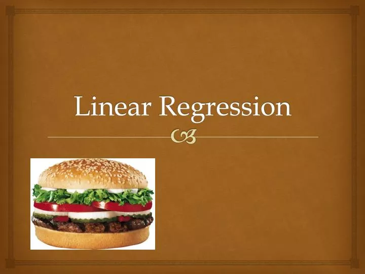
Linear Regression. The Whopper. One Double Whopper with cheese provides 53 grams of protein – all the protein you need in a day. It also supplies 1020 calories and 65 grams of fat. The Daily Value (based on a 2000-calorie diet) for fat is 65 grams.

E N D
The Whopper • One Double Whopper with cheese provides 53 grams of protein – all the protein you need in a day. • It also supplies 1020 calories and 65 grams of fat. The Daily Value (based on a 2000-calorie diet) for fat is 65 grams. • How are fat and protein related on the entire BK Menu? • The scatterplot for Fat (grams) vs. Protein (grams) shows a positive, moderately strong, linear relationship.
The Whopper The Whopper
Whopper, Association • So, if you want 25 grams of protein in your lunch, how much fat should you expect to consume at Burger King? • The correlation between fat and protein is .83, a sign that the linear association in the scatterplot is fairly strong. • However, strength of the relationship is only part of the picture. • The correlation says, “The linear association between these two variables is fairly strong” but it doesn’t tell us what the line is.
Let’s Say More • Yes, the relationship is strong, but let’s say something more: we can model the relationship with a line and give its equation • This equation will let us predict the fat content for any Burger King food, given its amount of protein. • How is this like what we do with a Normal Model?
Linear Model • A linear model is an equation of a straight line through the data. • Of course, no line can go through all the points, but a linear model can summarize the general pattern with only a couple of parameters. • Like all models of the real world, the model will be wrong – wrong in the sense that it cannot match reality exactly. But it can help us understand how these variables are associated.
Residuals • We want to find a line that goes through our data that comes closer to all the points than any other line. • It may turn out that this line doesn’t even hit a single point! But it does minimize the error between the line and each data point. • For one example, our line might predict the BK Broiled Chicken Sandwich with 30 grams of protein should have 36 grams of fat, when in fact, it actually has only 25 grams of fat. • We call the estimate made from a model the predicted valueand write it as which is called “y-hat” and distinguish it from the true value, y.
Residuals • The difference between the observed value, y, and the predicted value, , is called the residual. • The residual tells us how far off the model’s prediction is at that point. • The BK Broiled Chicken Residual would be g of fat. • To find residuals we always subtract the predicted value from the observed one.
Residuals • To find residuals we always subtract the predicted value from the observed one. • A negative residual means the predicted value is too big – an overestimate. • A positive residual shows that the model makes an underestimate.
“Best Fit” Means Least-Squares • When we draw our line through our scatter plot, some residuals are positive and some are negative. • We can’t assess how well the line fits by adding up all the residuals – the positive and negative ones will cancel each other out. • This is the same issue we faced when calculating Standard Deviation. • So what did we do?
Best Fit = Least Squares • We are going to square the residuals!!!!!!!!!!!!!!!!! • (Emphasis Added) • Squaring: Makes all the values positive Emphasizes the large residuals • The line of best fit is the line for which the sum of the squared residuals is smallest, the least squares line.
Finding That Line • What we know about correlation can lead us to the equation of the linear model. • Let’s look specifically at a scatterplot of standardized variables.
Finding the Line • Let’s start in the center of the plot – how much protein and fat does the typical Burger King food email provide? • The typical amount of protein content is What is the fat content of this average protein content? • The answer, as you might guess, is about average: • So…Our best fit line must go through the point . In the plot of z-scores, then, the line passes through the origin (0,0) • Why is that the case?
Finding the Line • A normal linear equation can be written in the form y=mx+b • If it passes through the origin, b=0, so the line can be expressed as y=mx where m is the slope of the line. • Note that our coordinates are not written (x,y) because they are z-scores, so our points are written and we need to indicate that the point on the line corresponding to a particular is :
Finding the Line • Now, many lines pass through the origin, but which one fits our data the best? • That is, which slope determines the line that minimizes the sum of squared residuals? • … • … • It turns out that the slope that minimizes our squared residuals is r itself!!!!!!!!!!!!!!!!!!!!!!!!!!!! • Once again, emphasis added.
Finding the Line • Wow! The equation for the line is about as simple as we could ever hope for: • What does it tell us? • It says that moving one standard deviation from the mean in x we can expect to move r standard deviations away from the mean in y.
Let’s get specific: For the sandwiches, the correlation is 0.83 If we standardize both protein and fat we can write: • This model tells us that for every standard deviation above (or below) the mean a sandwich is in protein, we’ll predict its fat content is 0.83 standard deviations above (or below) the mean fat content.
A double hamburger has 31 grams of protein, about 1 SD from the mean. • Putting 1.0 in for in the model gives a value of 0.83. If you trust the model, you’d expect the fat content to be about 0.83 fat SDs above the mean fat level. • Moving one standard deviation away from the mean in x moves our estimate r standard deviations away from the mean in y. • That is to say for our example, you’d expect the fat content to be about 0.83 fat SDs above the mean fat level.
R = 0, 1, or -1 • For r = 0, there is no linear relationship. The line is horizontal, and no matter how many standard deviations you move in x, the predicted value for y doesn’t change. • On the other hand, if r = 1.0 or -1.0, there’s a perfect linear association. In this case, moving one SD in x moves exactly the same number of SD in y.
How Big Can Predicted Values Get? • A new student is to join the class and you have to guess his height. • A reasonable guess would be to guess the mean height of male students in the class. • Now assume you are told he is 2 SDs above mean height in centimeters, how tall would you guess he is in inches? • Well, height in inches and height in centimeters are perfectly correlated, so you would guess 2 SDs in inches above the mean.
How Big Can Predicted Values Get? • A new student is to join the class and you have to guess his height. • A reasonable guess would be to guess the mean height of male students in the class. • Now assume you are told his GPA is 2 SDs above the mean. What would you guess his height to be? • There is little to no correlation between height and GPA so we would still guess the mean height of male students.
How Big Can Predicted Values Get? • A new student is to join the class and you have to guess his height. • A reasonable guess would be to guess the mean height of male students in the class. • Now, assume you are told he’s 2 SDs above the mean in shoe size. Now what would you guess his height to be? • There is a positive correlation between shoe size and height. We wouldn’t guess an exact correlation so it would be less than the 2 SDs we guessed from the height in centimeters example but it would certainly be higher than the 0 SD we guessed from the GPA example.
How Big Can Predicted Values Get? • The height example provides a key insight into a general rule: • Each predicted y value tends to be closer to its mean (in Standard Deviations) than its corresponding x value was. • The property of the linear model is called regression to the meanand the line is called the regression line.
Just Checking… • A scatterplot of house Price (in thousands of dollars) versus Size (in thousands of square feet) for houses sold recently in Saratoga Springs, NY shows a relationship that is straight, with only moderate scatter and no outliers. The correlation between house Price and Size is 0.77 • You go to an open house and find that the house is 1 SD above the mean in size. What would you expect about its price? • You read an ad for a house priced 2 SD below the mean. What would you guess about its size? • A friend tells you about a house whose size in square meters is 1.5 SD above the mean. What would you guess about its size in square feet?
Homework Page 192, # 1, 3, 5, 13, 15
The Regression Line in Real Units • We don’t always think in terms of z-scores, and in fact, most real world scenarios will require you keep thinking of things in their original units (though it is vital you understand the significance of their z-scores as well) • How much fat would you predict for a double hamburger with 31 grams of protein? • The mean for protein is near 17 grams and the SD is 14, so that items is1 SD above the mean. • Since r = 0.83, we predict the fat content will be 0.83 SD above the mean fat content.
The Regression Line in Real Units • Mean fat content is 23.5 grams and the SD for fat content is 16.4 grams, so we predict the double hamburger will have: • 23.5 + 0.83 * 16.4 = 37.11 grams of fat. • We can always convert both x and y to z-scores, find the correlation, use and then convert back to its original units so that we can understand the prediction. • But can this be done more simply?
The Regression Line in Real Units • Let’s re-write the equation of the line for protein and fat to be back in terms of the original units: • b0 is the y-intercept, the value of the line where it crosses the y-axis, and b1 is the slope • We find the slope using a formula developed on page 175-176 of your book, 0.93 grams of fat per gram of protein
The Regression Line in Real Units • Let’s re-write the equation of the line for protein and fat to be back in terms of the original units: • b0 is the y-intercept, the value of the line where it crosses the y-axis, and b1 is the slope • Next, how do we find the y-intercept ? Remember that the line has to go through the mean-mean point, ) • That is, the model predicts to be the value that corresponds to • We can put the means into the equation and write
The Regression Line in Real Units • Let’s re-write the equation of the line for protein and fat to be back in terms of the original units: • b0 is the y-intercept, the value of the line where it crosses the y-axis, and b1 is the slope • Rewrite to solve for gives us:
The Regression Line in Real Units • For our Burger King example this comes out to be
The Regression Line in Real Units Putting this back into the regression equation gives:
The Regression Line in Real Units The slope of 0.97 means that an additional gram of protein is associated with an additional 0.97grams of fat, on average. Less formally, we might say that BK sandwiches pack about 0.97 grams of fat per gram of protein. Keep in mind that for slope, units matter!
Slope and Units • The units of slope are always the units of y per units of x • Changing units doesn’t change the correlation but does change the standard deviations. The slope introduces the units into the equation by multiplying the correlation by the ratio of • If children grow an average of 3 inches per year that is the same as growing 0.21 millimeters per day.
The Intercept • What is the significance of the intercept of the BK regression line, 6.8? • This is the value of y when we are at an x of zero • So, for BK items, this means that we have 6.8 grams of fat even when an item contains noprotein.
Note! • When using a regression model it is vital that we check the same conditions for regressions as we did for correlation: • Quantitative Variable Condition • Straight Enough Condition • OutlierCondition