Download
1 / 24
240 likes | 349 Views
Geometrically motivated, hyperbolic gauge conditions for Numerical Relativity. Carlos Palenzuela Luque. 15 December 2005. -1-. Index. The coordinate degrees of freedom 1.1. The 3+1 decomposition 1.2. Definition of “good” coordinates for NR

E N D
Geometrically motivated, hyperbolic gauge conditions for Numerical Relativity Carlos Palenzuela Luque 15 December 2005 -1-
Index The coordinate degrees of freedom 1.1. The 3+1 decomposition 1.2. Definition of “good” coordinates for NR 2. Different gauge conditions 2.1. The harmonic coordinates 2.2. A driver to the minimal strain condition 2.3. Almost Stationary Motions 2.4. Comparations Numerical Tests -2-
1. THE COORDINATE DEGREES OF FREEDOM • Numerical Relativity: compute the metric gμν by solving • numerically the Einstein Equations (EE) Rμν – R gμν/ 2 = 8 πTμν μ,ν = 0, 1, 2, 3 • 10 Einstein Equations & 10 metric components gμν, but: • 4 coordinate degrees of freedom (gauge) one must prescribe 4 metric components • 4 equations are redundants (constraints) only 6 independent equations (evolution formalism) that fixes 6 metric components -3-
1. THE COORDINATE DEGREES OF FREEDOM1.1. The 3+1 decomposition (I) • Replace the 4D spacetime by a foliation (family of hypersurfaces) • Let us consider a congruence (family of curves) crossing the foliation, parametrized with t (t=cte also defines an hypersurface). • Let us define the following base of vectors: • ei: 3D base on the hypersurface • n: normal to the hypersurface • t: tangent to the curves of the congruence ∂t= α·n + βi·ei -4-
1. THE COORDINATE DEGREES OF FREEDOM1.1. The 3+1 decomposition (II) • The geometry of the manifold induced a intrinsic curvature in each hypersurface (i dt)·ei t + dt ∂t ·n ds2 = gμν dxμ dxν = - 2 dt2 + ij (dxi + idt)(dxj +jdt) ij t • EE provides evolution equations for the gij • Choosing the coordinates = fixing the time lines of the observers = fixing the lapse α and the shift βi = fixing g00 and g0i -5-
1.THE COORDINATE DEGREES OF FREEDOM1.2. “Good” coordinates for Numerical Relativity (I) 1) the evolution system (evolution formalism + gauge conditions) must be well posed –there is a solution and it is unique and stable- - in general is a difficult problem - the evolution formalism is basically hyperbolic (principal part similar to the wave equation) - find gauge conditions that preserve that hyperbolic character to the evolution system the well posedness of the problem is ensured -6-
1.THE COORDINATE DEGREES OF FREEDOM1.2. “Good” coordinates for Numerical Relativity (II) 2) the coordinates should be well adapted to stationary spacetimes, avoiding ficticious evolution due to the gauge. 3) the coordinate system should minimize some well defined geometrical quantities, taking advantage of the approximated symmetries of the problem - co-rotating frame in binary systems - asymptotically stationary spacetimes: black hole merging,.. -7-
2.DIFFERENT GAUGE CONDITIONS2.1. The harmonic coordinates (I) • Ensures the well posedness of the problem but does not have any geometrical meaning □ gμν - μ ν - ν μ = … Dedonder form of EE (4 const.) □ xμ = gσρμσρ = μ = 0 gauge condition □ gμν = … 6 evolution EE + 4 gauge conditions μ = 0 4 constraints ( □ is the Dedonder operator -wave operator in a curved spacetime-) -8-
2.DIFFERENT GAUGE CONDITIONS2.1. The harmonic coordinates (II) • Advantages: - the evolution system is well posed and the principal part is quite simple (decoupled wave equations) • Disadvantages: - the coordinate system does not have any geometrical motivation, so neither it is well adapted to stationary spacetimes nor minimize any geometrical quantity. -9-
2.DIFFERENT GAUGE CONDITIONS2.2. The driver to the minimal strain (I) 1) Let us define the strain Σij = ∂tγij 2) Construct the Lagrangian density L=ΣijΣij and its action S = ∫ L √γ dx3 3) Minimize this action with respect to the shift δS/δβi=0 kΣki =k [kβi + iβk + … ] = 0 • Minimal Strain : elliptic equation for the shift that is well adapted to stationary spacetimes and minimize the strain -10-
2.DIFFERENT GAUGE CONDITIONS2.2. The driver to the minimal strain (II) • Implement the elliptic equation by an hyperbolic driver (ie, convert the elliptic equation into an hyperbolic one) Example: Laplace equation kkφ = 0 hyperbolic driver ∂ttφ = kkφ – σ∂tφ • The solution of the hyperbolic driver tends to the solution of the elliptic equation for a range of values of the damping σ -11-
2.DIFFERENT GAUGE CONDITIONS2.2. The driver to the minimal strain (III) • Implement the minimal strain by an hyperbolic driver ti = - αQi , tQi +j ij = - σ Qi • It is a covariant generalization of the Gamma freezing ti = 2 j[1/3 ij] = 0 hyperbolic driver tQi + 2 j[1/3 ij] = - σ Qi -12-
2.DIFFERENT GAUGE CONDITIONS2.2. The driver to the minimal strain (IV) • Advantages: - the minimal strain shift driver have a geometrical motivation, so it is well adapted to stationary spacetimes and minimize the strain • Disadvantages: - the condition is implemented by an approximate driver - the lapse can not be obtained in the same way use another driver to the elliptic “maximal slicing” use the singularity avoidance Bona-Masso lapse equation (t - L) = - 2 f trK -13-
2.DIFFERENT GAUGE CONDITIONS2.3. The Almost Stationary Motions (I) • What do we want? (2) “ the coordinates should be well adapted to stationary spacetimes” stationary spacetime ∂t gμν = 0 Killing Equation ( = t) Lξ gμν = + = 0 • 10 equations for only 4 degrees of freedom ! not all the spacetimes admit Killing vectors -14-
2.DIFFERENT GAUGE CONDITIONS2.3. The Almost Stationary Motions (II) • Generalize the minimal strain condition to 4D: construct a Lagrangian density with the Killing Equation (;) = 0 L = (;) (;) - /2 (·)2 ( arbitrary parameter) and minimize this action S = ∫ L √g dx4 with respect to [(;) - /2 (·) g] = + R + (1-) (·) = 0 • The Almost Killing Equation (AKE) satisfies the Killing • equation and minimize the deviation from the isometries • the AKE defines a quasi-symmetry -15-
2. DIFFERENT GAUGE CONDITIONS2.3. The Almost Stationary Motions (III) • Let us consider the case λ = 1, where ξ is harmonic and the IVP is well posed (fixed background) Harmonic Almost Killing Equation (HAKE) + R = 0 [ 1/gL (g g) ] = 0 • Adapted coordinates = t - time lines as the integral curves of • - time as the preferred affine parameter g(t) = 0 -16-
2. DIFFERENT GAUGE CONDITIONS2.3. The Almost Stationary Motions (IV) • Advantages - the HAKE is well adapted to stationary spacetimes and minimize the deviation from the isometries t + 3 dt t + 2 dt KV t + dt ∂t t -17-
2. DIFFERENT GAUGE CONDITIONS2.3. The Almost Stationary Motions (V) • Advantages - the evolution system is well posed □gij - i j - j i = … (+ 4 constraints) t 0 = … (Provides the g00 component) t i = … (Provides the g0icomponents) • Triangular form. Characteristics along: • - time lines (Gamma sector) • - light cones (g sector) -18-
2. DIFFERENT GAUGE CONDITIONS2.3. The Almost Stationary Motions (VI) • Disadvantages - the system is weakly hyperbolic in the “luminal” points where the (coordinate) speed of light is zero (α=|βn|) it is only WH in a cone and not in all the directions numerically it still converges to the right solution - the lagrangian density is not positive definite common situation in GR: EE, geodesics,.. add damping terms to enforce the minimization tα = - α2Q , tQ= HAKE - σ Q ti = - αQi , tQi= HAKE - σ Qi -19-
One vector equation + R = 0 Adapted coords. g(t) = 0 Arbitrary space coords recombination xi= fi(yj) i,j = 1,2,3 (relabeling of time lines) 2. DIFFERENT GAUGE CONDITIONS2.4. Comparation: HAKE versus Harmonic coord. • Four scalar equations x = 0 • Adapted coords. g = 0 • Only linear (generic) combinations allowed -20-
3. NUMERICAL TESTS : the numerical code • Z4 evolution formalism: 10 equations for 10 variables R+ Z + Z = 8 ( T – T/2g ) • harmonic and HAKE gauge conditions • first order system (in space and time): first derivatives of the metric as independent quantities • finite difference code: Method of Lines with RK3 to evolve in time and spatial discrete difference operators satisfying Summation By Parts rule -22-
3. NUMERICAL TESTS: the Initial Data • Let us consider flat space-time in twisted coordinates x’ = x·[ 1 + A·sin(ω·x·y·z) ·exp(-r2/ε2)] y’ = y·[ 1 + A·sin(ω·x·y·z) ·exp(-r2/ε2)] z’ = z·[ 1 + A·sin(ω·x·y·z) ·exp(-r2/ε2)] • Set the lapse and the shift to the flat trivial values α = 1 , βi = 0 • The time lines are not aligned with the time Killing vector, so there will be a ficticious evolution due to the gauge • Let us consider a cubic domain xi= [-1/2, 1/2] with periodic boundary conditions -23-
3. NUMERICAL TESTS : Results 1. Play alpharm.mpeg the lapse with the harmonic 2. Play alpQ4.mpeg the same with the HAKE 3. Play bxharm.mpeg the shift (βx) with the harmonic 4. Play bxQ4.mpeg the same with the HAKE 5. Play Kxxharm.mpeg the Kxx with the harmonic 6. Play KxxQ4.mpeg the same with the HAKE The HAKE actually works! Try with BHs…. -24-